Polymath 8b, XI: Finishing up the paper

This is the eleventh thread for the Polymath8b project to obtain new bounds for the quantity

;

the previous thread may be found here.

The main focus is now on writing up the results, with a draft paper close to completion here (with the directory of source files here).    Most of the sections are now written up more or less completely, with the exception of the appendix on narrow admissible tuples, which was awaiting the bounds on such tuples to stabilise.  There is now also an acknowledgments section (linking to the corresponding page on the wiki, which participants should check to see if their affiliations etc. are posted correctly), and in the final remarks section there is now also some discussion about potential improvements to the bounds.  I’ve also added some mention of a recent paper of Banks, Freiberg and Maynard which makes use of some of our results (in particular, that ).  On the other hand, the portions of the writeup relating to potential improvements to the MPZ estimates have been commented out, as it appears that one cannot easily obtain the exponential sum estimates required to make those go through.  (Perhaps, if there are significant new developments, one could incorporate them into a putative Polymath8c project, although at present I think there’s not much urgency to start over once again.)

Regarding the numerics in Section 7 of the paper, one thing which is missing at present is some links to code in case future readers wish to verify the results; alternatively one could include such code and data into the arXiv submission.

It’s about time to discuss possible journals to submit the paper to.  Ken Ono has invited us to submit to his new journal, “Research in the Mathematical Sciences“.  Another option would be to submit to the same journal “Algebra & Number Theory” that is currently handling our Polymath8a paper (no news on the submission there, but it is a very long paper), although I think the papers are independent enough that it is not absolutely necessary to place them in the same journal.  A third natural choice is “Mathematics of Computation“, though I should note that when the Polymath4 paper was submitted there, the editors required us to use our real names instead of the D.H.J. Polymath pseudonym as it would have messed up their metadata system otherwise.  (But I can check with the editor there before submitting to see if there is some workaround now, perhaps their policies have changed.)  At present I have no strong preferences regarding journal selection, and would welcome further thoughts and proposals.  (It is perhaps best to avoid the journals that I am editor or associate editor of, namely Amer. J. Math, Forum of Mathematics, Analysis & PDE, and Dynamics and PDE, due to conflict of interest (and in the latter two cases, specialisation to a different area of mathematics)).

 

 

 

 

Kolmogorov’s power law for turbulence

Many fluid equations are expected to exhibit turbulence in their solutions, in which a significant portion of their energy ends up in high frequency modes. A typical example arises from the three-dimensional periodic Navier-Stokes equations

where is the velocity field, is a forcing term, is a pressure field, and is the viscosity. To study the dynamics of energy for this system, we first pass to the Fourier transform

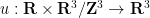
so that the system becomes

 

We may normalise (and ) to have mean zero, so that . Then we introduce the dyadic energies

where ranges over the powers of two, and is shorthand for . Taking the inner product of (1) with , we obtain the energy flow equation

 

where range over powers of two, is the energy flow rate

is the energy dissipation rate

and is the energy injection rate

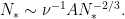
The Navier-Stokes equations are notoriously difficult to solve in general. Despite this, Kolmogorov in 1941 was able to give a convincing heuristic argument for what the distribution of the dyadic energies should become over long times, assuming that some sort of distributional steady state is reached. It is common to present this argument in the form of dimensional analysis, but one can also give a more “first principles” form Kolmogorov’s argument, which I will do here. Heuristically, one can divide the frequency scales into three regimes:

• The injection regime in which the energy injection rate dominates the right-hand side of (2);
• The energy flow regime in which the flow rates dominate the right-hand side of (2); and
• The dissipation regime in which the dissipation dominates the right-hand side of (2).

If we assume a fairly steady and smooth forcing term , then will be supported on the low frequency modes , and so we heuristically expect the injection regime to consist of the low scales . Conversely, if we take the viscosity to be small, we expect the dissipation regime to only occur for very large frequencies , with the energy flow regime occupying the intermediate frequencies.

We can heuristically predict the dividing line between the energy flow regime. Of all the flow rates , it turns out in practice that the terms in which (i.e., interactions between comparable scales, rather than widely separated scales) will dominate the other flow rates, so we will focus just on these terms. It is convenient to return back to physical space, decomposing the velocity field into Littlewood-Paley components

of the velocity field at frequency . By Plancherel’s theorem, this field will have an norm of , and as a naive model of turbulence we expect this field to be spread out more or less uniformly on the torus, so we have the heuristic

and a similar heuristic applied to gives

(One can consider modifications of the Kolmogorov model in which is concentrated on a lower-dimensional subset of the three-dimensional torus, leading to some changes in the numerology below, but we will not consider such variants here.) Since

we thus arrive at the heuristic

Of course, there is the possibility that due to significant cancellation, the energy flow is significantly less than , but we will assume that cancellation effects are not that significant, so that we typically have

 

or (assuming that does not oscillate too much in , and are close to )

On the other hand, we clearly have

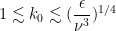
We thus expect to be in the dissipation regime when

 

and in the energy flow regime when

 

Now we study the energy flow regime further. We assume a “statistically scale-invariant” dynamics in this regime, in particular assuming a power law

 

for some . From (3), we then expect an average asymptotic of the form

 

for some structure constants that depend on the exact nature of the turbulence; here we have replaced the factor by the comparable term to make things more symmetric. In order to attain a steady state in the energy flow regime, we thus need a cancellation in the structure constants:

 

On the other hand, if one is assuming statistical scale invariance, we expect the structure constants to be scale-invariant (in the energy flow regime), in that

 

for dyadic . Also, since the Euler equations conserve energy, the energy flows symmetrise to zero,

which from (7) suggests a similar cancellation among the structure constants

Combining this with the scale-invariance (9), we see that for fixed , we may organise the structure constants for dyadic into sextuples which sum to zero (including some degenerate tuples of order less than six). This will automatically guarantee the cancellation (8) required for a steady state energy distribution, provided that

or in other words

for any other value of , there is no particular reason to expect this cancellation (8) to hold. Thus we are led to the heuristic conclusion that the most stable power law distribution for the energies is the law

 

or in terms of shell energies, we have the famous Kolmogorov 5/3 law

Given that frequency interactions tend to cascade from low frequencies to high (if only because there are so many more high frequencies than low ones), the above analysis predicts a stablising effect around this power law: scales at which a law (6) holds for some are likely to lose energy in the near-term, while scales at which a law (6) hold for some are conversely expected to gain energy, thus nudging the exponent of power law towards .

We can solve for in terms of energy dissipation as follows. If we let be the frequency scale demarcating the transition from the energy flow regime (5) to the dissipation regime (4), we have

and hence by (10)

On the other hand, if we let be the energy dissipation at this scale (which we expect to be the dominant scale of energy dissipation), we have

Some simple algebra then lets us solve for and as

and

Thus, we have the Kolmogorov prediction

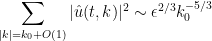
for

with energy dissipation occuring at the high end of this scale, which is counterbalanced by the energy injection at the low end of the scale.

Dwork’s proof of rationality of the zeta function over finite fields

Let be a quasiprojective variety defined over a finite field , thus for instance could be an affine variety

where is -dimensional affine space and are a finite collection of polynomials with coefficients in . Then one can define the set of -rational points, and more generally the set of -rational points for any , since can be viewed as a field extension of . Thus for instance in the affine case (1) we have

The Weil conjectures are concerned with understanding the number

of -rational points over a variety . The first of these conjectures was proven by Dwork, and can be phrased as follows.

Theorem 1 (Rationality of the zeta function) Let be a quasiprojective variety defined over a finite field , and let be given by (2). Then there exist a finite number of algebraic integers (known as characteristic values of ), such that

for all .

After cancelling, we may of course assume that for any and , and then it is easy to see (as we will see below) that the become uniquely determined up to permutations of the and . These values are known as the characteristic values of . Since is a rational integer (i.e. an element of ) rather than merely an algebraic integer (i.e. an element of the ring of integers of the algebraic closure of ), we conclude from the above-mentioned uniqueness that the set of characteristic values are invariant with respect to the Galois group . To emphasise this Galois invariance, we will not fix a specific embedding of the algebraic numbers into the complex field , but work with all such embeddings simultaneously. (Thus, for instance, contains three cube roots of , but which of these is assigned to the complex numbers , , will depend on the choice of embedding .)

An equivalent way of phrasing Dwork’s theorem is that the (-form of the) zeta function

associated to (which is well defined as a formal power series in , at least) is equal to a rational function of (with the and being the poles and zeroes of respectively). Here, we use the formal exponential

Equivalently, the (-form of the) zeta-function is a meromorphic function on the complex numbers which is also periodic with period , and which has only finitely many poles and zeroes up to this periodicity.

Dwork’s argument relies primarily on -adic analysis – an analogue of complex analysis, but over an algebraically complete (and metrically complete) extension of the -adic field , rather than over the Archimedean complex numbers . The argument is quite effective, and in particular gives explicit upper bounds for the number of characteristic values in terms of the complexity of the variety ; for instance, in the affine case (1) with of degree , Bombieri used Dwork’s methods (in combination with Deligne’s theorem below) to obtain the bound , and a subsequent paper of Hooley established the slightly weaker bound purely from Dwork’s methods (a similar bound had also been pointed out in unpublished work of Dwork). In particular, one has bounds that are uniform in the field , which is an important fact for many analytic number theory applications.

These -adic arguments stand in contrast with Deligne’s resolution of the last (and deepest) of the Weil conjectures:

Theorem 2 (Riemann hypothesis) Let be a quasiprojective variety defined over a finite field , and let be a characteristic value of . Then there exists a natural number such that for every embedding , where denotes the usual absolute value on the complex numbers . (Informally: and all of its Galois conjugates have complex magnitude .)

To put it another way that closely resembles the classical Riemann hypothesis, all the zeroes and poles of the -form lie on the critical lines for . (See this previous blog post for further comparison of various instantiations of the Riemann hypothesis.) Whereas Dwork uses -adic analysis, Deligne uses the essentially orthogonal technique of ell-adic cohomology to establish his theorem. However, ell-adic methods can be used (via the Grothendieck-Lefschetz trace formula) to establish rationality, and conversely, in this paper of Kedlaya p-adic methods are used to establish the Riemann hypothesis. As pointed out by Kedlaya, the ell-adic methods are tied to the intrinsic geometry of (such as the structure of sheaves and covers over ), while the -adic methods are more tied to the extrinsic geometry of (how sits inside its ambient affine or projective space).

In this post, I would like to record my notes on Dwork’s proof of Theorem 1, drawing heavily on the expositions of Serre, Hooley, Koblitz, and others.

The basic strategy is to control the rational integers both in an “Archimedean” sense (embedding the rational integers inside the complex numbers with the usual norm ) as well as in the “-adic” sense, with the characteristic of (embedding the integers now in the “complexification” of the -adic numbers , which is equipped with a norm that we will recall later). (This is in contrast to the methods of ell-adic cohomology, in which one primarily works over an -adic field with .) The Archimedean control is trivial:

Proposition 3 (Archimedean control of ) With as above, and any embedding , we have

for all and some independent of .

Proof: Since is a rational integer, is just . By decomposing into affine pieces, we may assume that is of the affine form (1), then we trivially have , and the claim follows.

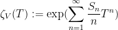
Another way of thinking about this Archimedean control is that it guarantees that the zeta function can be defined holomorphically on the open disk in of radius centred at the origin.

The -adic control is significantly more difficult, and is the main component of Dwork’s argument:

Proposition 4 (-adic control of ) With as above, and using an embedding (defined later) with the characteristic of , we can find for any real a finite number of elements such that

for all .

Another way of thinking about this -adic control is that it guarantees that the zeta function can be defined meromorphically on the entire -adic complex field .

Proposition 4 is ostensibly much weaker than Theorem 1 because of (a) the error term of -adic magnitude at most ; (b) the fact that the number of potential characteristic values here may go to infinity as ; and (c) the potential characteristic values only exist inside the complexified -adics , rather than in the algebraic integers . However, it turns out that by combining -adic control on in Proposition 4 with the trivial control on in Proposition 3, one can obtain Theorem 1 by an elementary argument that does not use any further properties of (other than the obvious fact that the are rational integers), with the in Proposition 4 chosen to exceed the in Proposition 3. We give this argument (essentially due to Borel) below the fold.

The proof of Proposition 4 can be split into two pieces. The first piece, which can be viewed as the number-theoretic component of the proof, uses external descriptions of such as (1) to obtain the following decomposition of :

Proposition 5 (Decomposition of ) With and as above, we can decompose as a finite linear combination (over the integers) of sequences , such that for each such sequence , the zeta functions

are entire in , by which we mean that

as .

This proposition will ultimately be a consequence of the properties of the Teichmuller lifting .

The second piece, which can be viewed as the “-adic complex analytic” component of the proof, relates the -adic entire nature of a zeta function with control on the associated sequence , and can be interpreted (after some manipulation) as a -adic version of the Weierstrass preparation theorem:

Proposition 6 (-adic Weierstrass preparation theorem) Let be a sequence in , such that the zeta function

is entire in . Then for any real , there exist a finite number of elements such that

for all and some .

Clearly, the combination of Proposition 5 and Proposition 6 (and the non-Archimedean nature of the norm) imply Proposition 4.

Stickiness, graininess, planiness, and a sum-product approach to the Kakeya problem

This is a blog version of a talk I recently gave at the IPAM workshop on “The Kakeya Problem, Restriction Problem, and Sum-product Theory”.

Note: the discussion here will be highly non-rigorous in nature, being extremely loose in particular with asymptotic notation and with the notion of dimension. Caveat emptor.

One of the most infamous unsolved problems at the intersection of geometric measure theory, incidence combinatorics, and real-variable harmonic analysis is the Kakeya set conjecture. We will focus on the following three-dimensional case of the conjecture, stated informally as follows:

Conjecture 1 (Kakeya conjecture) Let be a subset of that contains a unit line segment in every direction. Then .

This conjecture is not precisely formulated here, because we have not specified exactly what type of set is (e.g. measurable, Borel, compact, etc.) and what notion of dimension we are using. We will deliberately ignore these technical details in this post. It is slightly more convenient for us here to work with lines instead of unit line segments, so we work with the following slight variant of the conjecture (which is essentially equivalent):

Conjecture 2 (Kakeya conjecture, again) Let be a family of lines in that meet and contain a line in each direction. Let be the union of the restriction to of every line in . Then .

As the space of all directions in is two-dimensional, we thus see that is an (at least) two-dimensional subset of the four-dimensional space of lines in (actually, it lies in a compact subset of this space, since we have constrained the lines to meet ). One could then ask if this is the only property of that is needed to establish the Kakeya conjecture, that is to say if any subset of which contains a two-dimensional family of lines (restricted to , and meeting ) is necessarily three-dimensional. Here we have an easy counterexample, namely a plane in (passing through the origin), which contains a two-dimensional collection of lines. However, we can exclude this case by adding an additional axiom, leading to what one might call a “strong” Kakeya conjecture:

Conjecture 3 (Strong Kakeya conjecture) Let be a two-dimensional family of lines in that meet , and assume the Wolff axiom that no (affine) plane contains more than a one-dimensional family of lines in . Let be the union of the restriction of every line in . Then .

Actually, to make things work out we need a more quantitative version of the Wolff axiom in which we constrain the metric entropy (and not just dimension) of lines that lie close to a plane, rather than exactly on the plane. However, for the informal discussion here we will ignore these technical details. Families of lines that lie in different directions will obey the Wolff axiom, but the converse is not true in general.

In 1995, Wolff established the important lower bound (for various notions of dimension, e.g. Hausdorff dimension) for sets in Conjecture 3 (and hence also for the other forms of the Kakeya problem). However, there is a key obstruction to going beyond the barrier, coming from the possible existence of half-dimensional (approximate) subfields of the reals . To explain this problem, it easiest to first discuss the complex version of the strong Kakeya conjecture, in which all relevant (real) dimensions are doubled:

Conjecture 4 (Strong Kakeya conjecture over ) Let be a four (real) dimensional family of complex lines in that meet the unit ball in , and assume the Wolff axiom that no four (real) dimensional (affine) subspace contains more than a two (real) dimensional family of complex lines in . Let be the union of the restriction of every complex line in . Then has real dimension .

The argument of Wolff can be adapted to the complex case to show that all sets occuring in Conjecture 4 have real dimension at least . Unfortunately, this is sharp, due to the following fundamental counterexample:

Proposition 5 (Heisenberg group counterexample) Let be the Heisenberg group

and let be the family of complex lines

with and . Then is a five (real) dimensional subset of that contains every line in the four (real) dimensional set ; however each four real dimensional (affine) subspace contains at most a two (real) dimensional set of lines in . In particular, the strong Kakeya conjecture over the complex numbers is false.

This proposition is proven by a routine computation, which we omit here. The group structure on is given by the group law

giving the structure of a -step simply-connected nilpotent Lie group, isomorphic to the usual Heisenberg group over . Note that while the Heisenberg group is a counterexample to the complex strong Kakeya conjecture, it is not a counterexample to the complex form of the original Kakeya conjecture, because the complex lines in the Heisenberg counterexample do not point in distinct directions, but instead only point in a three (real) dimensional subset of the four (real) dimensional space of available directions for complex lines. For instance, one has the one real-dimensional family of parallel lines

with ; multiplying this family of lines on the right by a group element in gives other families of parallel lines, which in fact sweep out all of .

The Heisenberg counterexample ultimately arises from the “half-dimensional” (and hence degree two) subfield of , which induces an involution which can then be used to define the Heisenberg group through the formula

Analogous Heisenberg counterexamples can also be constructed if one works over finite fields that contain a “half-dimensional” subfield ; we leave the details to the interested reader. Morally speaking, if in turn contained a subfield of dimension (or even a subring or “approximate subring”), then one ought to be able to use this field to generate a counterexample to the strong Kakeya conjecture over the reals. Fortunately, such subfields do not exist; this was a conjecture of Erdos and Volkmann that was proven by Edgar and Miller, and more quantitatively by Bourgain (answering a question of Nets Katz and myself). However, this fact is not entirely trivial to prove, being a key example of the sum-product phenomenon.

We thus see that to go beyond the dimension bound of Wolff for the 3D Kakeya problem over the reals, one must do at least one of two things:

• (a) Exploit the distinct directions of the lines in in a way that goes beyond the Wolff axiom; or
• (b) Exploit the fact that does not contain half-dimensional subfields (or more generally, intermediate-dimensional approximate subrings).

(The situation is more complicated in higher dimensions, as there are more obstructions than the Heisenberg group; for instance, in four dimensions quadric surfaces are an important obstruction, as discussed in this paper of mine.)

Various partial or complete results on the Kakeya problem over various fields have been obtained through route (a) or route (b). For instance, in 2000, Nets Katz, Izabella Laba and myself used route (a) to improve Wolff’s lower bound of for Kakeya sets very slightly to (for a weak notion of dimension, namely upper Minkowski dimension). In 2004, Bourgain, Katz, and myself established a sum-product estimate which (among other things) ruled out approximate intermediate-dimensional subrings of , and then pursued route (b) to obtain a corresponding improvement to the Kakeya conjecture over finite fields of prime order. The analogous (discretised) sum-product estimate over the reals was established by Bourgain in 2003, which in principle would allow one to extend the result of Katz, Laba and myself to the strong Kakeya setting, but this has not been carried out in the literature. Finally, in 2009, Dvir used route (a) and introduced the polynomial method (as discussed previously here) to completely settle the Kakeya conjecture in finite fields.

Below the fold, I present a heuristic argument of Nets Katz and myself, which in principle would use route (b) to establish the full (strong) Kakeya conjecture. In broad terms, the strategy is as follows:

1. Assume that the (strong) Kakeya conjecture fails, so that there are sets of the form in Conjecture 3 of dimension for some . Assume that is “optimal”, in the sense that is as large as possible.
2. Use the optimality of (and suitable non-isotropic rescalings) to establish strong forms of standard structural properties expected of such sets , namely “stickiness”, “planiness”, “local graininess” and “global graininess” (we will roughly describe these properties below). Heuristically, these properties are constraining to “behave like” a putative Heisenberg group counterexample.
3. By playing all these structural properties off of each other, show that can be parameterised locally by a one-dimensional set which generates a counterexample to Bourgain’s sum-product theorem. This contradiction establishes the Kakeya conjecture.

Nets and I have had an informal version of argument for many years, but were never able to make a satisfactory theorem (or even a partial Kakeya result) out of it, because we could not rigorously establish anywhere near enough of the necessary structural properties (stickiness, planiness, etc.) on the optimal set for a large number of reasons (one of which being that we did not have a good notion of dimension that did everything that we wished to demand of it). However, there is beginning to be movement in these directions (e.g. in this recent result of Guth using the polynomial method obtaining a weak version of local graininess on certain Kakeya sets). In view of this (and given that neither Nets or I have been actively working in this direction for some time now, due to many other projects), we’ve decided to distribute these ideas more widely than before, and in particular on this blog.

The Bombieri-Stepanov proof of the Hasse-Weil bound

Let be a finite field of order , and let be an absolutely irreducible smooth projective curve defined over (and hence over the algebraic closure of that field). For instance, could be the projective elliptic curve

in the projective plane , where are coefficients whose discriminant is non-vanishing, which is the projective version of the affine elliptic curve

To each such curve one can associate a genus , which we will define later; for instance, elliptic curves have genus . We can also count the cardinality of the set of -points of . The Hasse-Weil bound relates the two:

Theorem 1 (Hasse-Weil bound) .

The usual proofs of this bound proceed by first establishing a trace formula of the form

 

for some complex numbers independent of ; this is in fact a special case of the Lefschetz-Grothendieck trace formula, and can be interpreted as an assertion that the zeta function associated to the curve is rational. The task is then to establish a bound for all ; this (or more precisely, the slightly stronger assertion ) is the Riemann hypothesis for such curves. This can be done either by passing to the Jacobian variety of and using a certain duality available on the cohomology of such varieties, known as Rosati involution; alternatively, one can pass to the product surface and apply the Riemann-Roch theorem for that surface.

In 1969, Stepanov introduced an elementary method (a version of what is now known as the polynomial method) to count (or at least to upper bound) the quantity . The method was initially restricted to hyperelliptic curves, but was soon extended to general curves. In particular, Bombieri used this method to give a short proof of the following weaker version of the Hasse-Weil bound:

Theorem 2 (Weak Hasse-Weil bound) If is a perfect square, and , then .

In fact, the bound on can be sharpened a little bit further, as we will soon see.

Theorem 2 is only an upper bound on , but there is a Galois-theoretic trick to convert (a slight generalisation of) this upper bound to a matching lower bound, and if one then uses the trace formula (1) (and the “tensor power trick” of sending to infinity to control the weights ) one can then recover the full Hasse-Weil bound. We discuss these steps below the fold.

I’ve discussed Bombieri’s proof of Theorem 2 in this previous post (in the special case of hyperelliptic curves), but now wish to present the full proof, with some minor simplifications from Bombieri’s original presentation; it is mostly elementary, with the deepest fact from algebraic geometry needed being Riemann’s inequality (a weak form of the Riemann-Roch theorem).

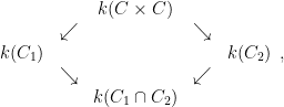
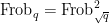
The first step is to reinterpret as the number of points of intersection between two curves in the surface . Indeed, if we define the Frobenius endomorphism on any projective space by

then this map preserves the curve , and the fixed points of this map are precisely the points of :

Thus one can interpret as the number of points of intersection between the diagonal curve

and the Frobenius graph

which are copies of inside . But we can use the additional hypothesis that is a perfect square to write this more symmetrically, by taking advantage of the fact that the Frobenius map has a square root

with also preserving . One can then also interpret as the number of points of intersection between the curve

 

and its transpose

Let be the field of rational functions on (with coefficients in ), and define , , and analogously )(although is likely to be disconnected, so will just be a ring rather than a field. We then (morally) have the commuting square

if we ignore the issue that a rational function on, say, , might blow up on all of and thus not have a well-defined restriction to . We use and to denote the restriction maps. Furthermore, we have obvious isomorphisms , coming from composing with the graphing maps and .

The idea now is to find a rational function on the surface of controlled degree which vanishes when restricted to , but is non-vanishing (and not blowing up) when restricted to . On , we thus get a non-zero rational function of controlled degree which vanishes on – which then lets us bound the cardinality of in terms of the degree of . (In Bombieri’s original argument, one required vanishing to high order on the side, but in our presentation, we have factored out a term which removes this high order vanishing condition.)

To find this , we will use linear algebra. Namely, we will locate a finite-dimensional subspace of (consisting of certain “controlled degree” rational functions) which projects injectively to , but whose projection to has strictly smaller dimension than itself. The rank-nullity theorem then forces the existence of a non-zero element of whose projection to vanishes, but whose projection to is non-zero.

Now we build . Pick a point of , which we will think of as being a point at infinity. (For the purposes of proving Theorem 2, we may clearly assume that is non-empty.) Thus is fixed by . To simplify the exposition, we will also assume that is fixed by the square root of ; in the opposite case when has order two when acting on , the argument is essentially the same, but all references to in the second factor of need to be replaced by (we leave the details to the interested reader).

For any natural number , define to be the set of rational functions which are allowed to have a pole of order up to at , but have no other poles on ; note that as we are assuming to be smooth, it is unambiguous what a pole is (and what order it will have). (In the fancier language of divisors and Cech cohomology, we have .) The space is clearly a vector space over ; one can view intuitively as the space of “polynomials” on of “degree” at most . When , consists just of the constant functions. Indeed, if , then the image of avoids and so lies in the affine line ; but as is projective, the image needs to be compact (hence closed) in , and must therefore be a point, giving the claim.

For higher , we have the easy relations

 

The former inequality just comes from the trivial inclusion . For the latter, observe that if two functions lie in , so that they each have a pole of order at most at , then some linear combination of these functions must have a pole of order at most at ; thus has codimension at most one in , giving the claim.

From (3) and induction we see that each of the are finite dimensional, with the trivial upper bound

 

Riemann’s inequality complements this with the lower bound

 

thus one has for all but at most exceptions (in fact, exactly exceptions as it turns out). This is a consequence of the Riemann-Roch theorem; it can be proven from abstract nonsense (the snake lemma) if one defines the genus in a non-standard fashion (as the dimension of the first Cech cohomology of the structure sheaf of ), but to obtain this inequality with a standard definition of (e.g. as the dimension of the zeroth Cech cohomolgy of the line bundle of differentials) requires the more non-trivial tool of Serre duality.

At any rate, now that we have these vector spaces , we will define to be a tensor product space

for some natural numbers which we will optimise in later. That is to say, is spanned by functions of the form with and . This is clearly a linear subspace of of dimension , and hence by Rieman’s inequality we have

 

if

 

Observe that maps a tensor product to a function . If and , then we see that the function has a pole of order at most at . We conclude that

 

and in particular by (4)

 

and similarly

 

We will choose to be a bit bigger than , to make the image of smaller than that of . From (6), (10) we see that if we have the inequality

 

(together with (7)) then cannot be injective.

On the other hand, we have the following basic fact:

Lemma 3 (Injectivity) If

 

then is injective.

Proof: From (3), we can find a linear basis of such that each of the has a distinct order of pole at (somewhere between and inclusive). Similarly, we may find a linear basis of such that each of the has a distinct order of pole at (somewhere between and inclusive). The functions then span , and the order of pole at is . But since , these orders are all distinct, and so these functions must be linearly independent. The claim follows.

This gives us the following bound:

Proposition 4 Let be natural numbers such that (7), (11), (12) hold. Then .

Proof: As is not injective, we can find with vanishing. By the above lemma, the function is then non-zero, but it must also vanish on , which has cardinality . On the other hand, by (8), has a pole of order at most at and no other poles. Since the number of poles and zeroes of a rational function on a projective curve must add up to zero, the claim follows.

If , we may make the explicit choice

and a brief calculation then gives Theorem 2. In some cases one can optimise things a bit further. For instance, in the genus zero case (e.g. if is just the projective line ) one may take and conclude the absolutely sharp bound in this case; in the case of the projective line , the function is in fact the very concrete function .

Remark 1 When is not a perfect square, one can try to run the above argument using the factorisation instead of . This gives a weaker version of the above bound, of the shape . In the hyperelliptic case at least, one can erase this loss by working with a variant of the argument in which one requires to vanish to high order at , rather than just to first order; see this survey article of mine for details.