AI Mathematical Olympiad – Progress Prize Competition now open

The first progress prize competition for the AI Mathematical Olympiad has now launched. (Disclosure: I am on the advisory committee for the prize.) This is a competition in which contestants submit an AI model which, after the submissions deadline on June 27, will be tested (on a fixed computational resource, without internet access) on a set of 50 “private” test math problems, each of which has an answer as an integer between 0 and 999. Prior to the close of submission, the models can be tested on 50 “public” test math problems (where the results of the model are public, but not the problems themselves), as well as 10 training problems that are available to all contestants. As of this time of writing, the leaderboard shows that the best-performing model has solved 4 out of 50 of the questions (a standard benchmark, Gemma 7B, had previously solved 3 out of 50). A total of $ ($1.048 million) has been allocated for various prizes associated to this competition. More detailed rules can be found here.

Illustrating the Impact of the Mathematical Sciences

Over the last few years, I have served on a committee of the National Academy of Sciences to produce some posters and other related media to showcase twenty-first century and its applications in the real world, suitable for display in classrooms or math departments. Our posters (together with some associated commentary, webinars on related topics, and even a whimsical “comic“) are now available for download here.

The spherical Cayley-Menger determinant and the radius of the Earth

Given three points in the plane, the distances between them have to be non-negative and obey the triangle inequalities

but are otherwise unconstrained. But if one has four points in the plane, then there is an additional constraint connecting the six distances between them, coming from the Cayley-Menger determinant:

Proposition 1 (Cayley-Menger determinant) If are four points in the plane, then the Cayley-Menger determinant

vanishes.

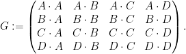
Proof: If we view as vectors in , then we have the usual cosine rule , and similarly for all the other distances. The matrix appearing in (1) can then be written as , where is the matrix

and is the (augmented) Gram matrix

The matrix is a rank one matrix, and so is also. The Gram matrix factorises as , where is the matrix with rows , and thus has rank at most . Therefore the matrix in (1) has rank at most , and hence has determinant zero as claimed.

For instance, if we know that and , then in order for to be coplanar, the remaining distance has to obey the equation

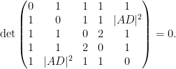
After some calculation the left-hand side simplifies to , so the non-negative quantity is constrained to equal either or . The former happens when form a unit right-angled triangle with right angle at and ; the latter happens when form the vertices of a unit square traversed in that order. Any other value for is not compatible with the hypothesis for lying on a plane; hence the Cayley-Menger determinant can be used as a test for planarity.

Now suppose that we have four points on a sphere of radius , with six distances now measured as lengths of arcs on the sphere. There is a spherical analogue of the Cayley-Menger determinant:

Proposition 2 (Spherical Cayley-Menger determinant) If are four points on a sphere of radius in , then the spherical Cayley-Menger determinant

vanishes.

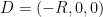
Proof: We can assume that the sphere is centred at the origin of , and view as vectors in of magnitude . The angle subtended by from the origin is , so by the cosine rule we have

Similarly for all the other inner products. Thus the matrix in (2) can be written as , where is the Gram matrix

We can factor where is the matrix with rows . Thus has rank at most and thus the determinant vanishes as required.

Just as the Cayley-Menger determinant can be used to test for coplanarity, the spherical Cayley-Menger determinant can be used to test for lying on a sphere of radius . For instance, if we know that lie on and are all equal to , then the above proposition gives

The left-hand side evaluates to ; as lies between and , the only choices for this distance are then and . The former happens for instance when lies on the north pole , are points on the equator with longitudes differing by 90 degrees, and is also equal to the north pole; the latter occurs when is instead placed on the south pole.

The Cayley-Menger and spherical Cayley-Menger determinants look slightly different from each other, but one can transform the latter into something resembling the former by row and column operations. Indeed, the determinant (2) can be rewritten as

and by further row and column operations, this determinant vanishes if and only if the determinant

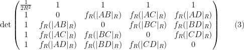
vanishes, where 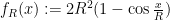. In the limit (so that the curvature of the sphere tends to zero), tends to , and by Taylor expansion tends to ; similarly for the other distances. Now we see that the planar Cayley-Menger determinant emerges as the limit of (3) as , as would be expected from the intuition that a plane is essentially a sphere of infinite radius.

In principle, one can now estimate the radius of the Earth (assuming that it is either a sphere or a flat plane ) if one is given the six distances between four points on the Earth. Of course, if one wishes to do so, one should have rather far apart from each other, since otherwise it would be difficult to for instance distinguish the round Earth from a flat one. As an experiment, and just for fun, I wanted to see how accurate this would be with some real world data. I decided to take , , , be the cities of London, Los Angeles, Tokyo, and Dubai respectively. As an initial test, I used distances from this online flight calculator, measured in kilometers:

Given that the true radius of the earth was about kilometers, I chose the change of variables (so that corresponds to the round Earth model with the commonly accepted value for the Earth’s radius, and corresponds to the flat Earth), and obtained the following plot for (3):

In particular, the determinant does indeed come very close to vanishing when , which is unsurprising since, as explained on the web site, the online flight calculator uses a model in which the Earth is an ellipsoid of radii close to km. There is another radius that would also be compatible with this data at (corresponding to an Earth of radius about km), but presumably one could rule out this as a spurious coincidence by experimenting with other quadruples of cities than the ones I selected. On the other hand, these distances are highly incompatible with the flat Earth model ; one could also see this with a piece of paper and a ruler by trying to lay down four points on the paper with (an appropriately rescaled) version of the above distances (e.g., with , , etc.).

If instead one goes to the flight time calculator and uses flight travel times instead of distances, one now gets the following data (measured in hours):

Assuming that planes travel at about kilometers per hour, the true radius of the Earth should be about of flight time. If one then uses the normalisation , one obtains the following plot:

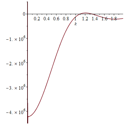
Not too surprisingly, this is basically a rescaled version of the previous plot, with vanishing near and at . (The website for the flight calculator does say it calculates short and long haul flight times slightly differently, which may be the cause of the slight discrepancies between this figure and the previous one.)

Of course, these two data sets are “cheating” since they come from a model which already presupposes what the radius of the Earth is. But one can input real world flight times between these four cities instead of the above idealised data. Here one runs into the issue that the flight time from to is not necessarily the same as that from to due to such factors as windspeed. For instance, I looked up the online flight time from Tokyo to Dubai to be 11 hours and 10 minutes, whereas the online flight time from Dubai to Tokyo was 9 hours and 50 minutes. The simplest thing to do here is take an arithmetic mean of the two times as a preliminary estimate for the flight time without windspeed factors, thus for instance the Tokyo-Dubai flight time would now be 10 hours and 30 minutes, and more generally

This data is not too far off from the online calculator data, but it does distort the graph slightly (taking as before):

Now one gets estimates for the radius of the Earth that are off by about a factor of from the truth, although the round Earth model still is twice as accurate as the flat Earth model .

Given that windspeed should additively affect flight velocity rather than flight time, and the two are inversely proportional to each other, it is more natural to take a harmonic mean rather than an arithmetic mean. This gives the slightly different values

but one still gets essentially the same plot:

So the inaccuracies are presumably coming from some other source. (Note for instance that the true flight time from Tokyo to Dubai is about greater than the calculator predicts, while the flight time from LA to Dubai is about less; these sorts of errors seem to pile up in this calculation.) Nevertheless, it does seem that flight time data is (barely) enough to establish the roundness of the Earth and obtain a somewhat ballpark estimate for its radius. (I assume that the fit would be better if one could include some Southern Hemisphere cities such as Sydney or Santiago, but I was not able to find a good quadruple of widely spaced cities on both hemispheres for which there were direct flights between all six pairs.)

Two announcements

Now that Google Plus is closing, the brief announcements that I used to post over there will now be migrated over to this blog.  (Some people have suggested other platforms for this also, such as Twitter, but I think for now I can use my existing blog to accommodate these sorts of short posts.)

1. The NSF-CBMS regional research conferences are now requesting proposals for the 2020 conference series.  (I was the principal lecturer for one of these conferences back in 2005; it was a very intensive experience, but quite enjoyable, and I am quite pleased with the book that resulted from it.)
2. The awardees for the Sloan Fellowships for 2019 have now been announced.  (I was on the committee for the mathematics awards.  For the usual reasons involving the confidentiality of letters of reference and other sensitive information, I will be unfortunately be unable to answer any specific questions about our committee deliberations.)

Request for comments from the ICM Structure Committee

[This post is collectively authored by the ICM structure committee, whom I am currently chairing – T.]

The International Congress of Mathematicians (ICM) is widely considered to be the premier conference for mathematicians.  It is held every four years; for instance, the 2018 ICM was held in Rio de Janeiro, Brazil, and the 2022 ICM is to be held in Saint Petersburg, Russia.  The most high-profile event at the ICM is the awarding of the 10 or so prizes of the International Mathematical Union (IMU) such as the Fields Medal, and the lectures by the prize laureates; but there are also approximately twenty plenary lectures from leading experts across all mathematical disciplines, several public lectures of a less technical nature, about 180 more specialised invited lectures divided into about twenty section panels, each corresponding to a mathematical field (or range of fields), as well as various outreach and social activities, exhibits and satellite programs, and meetings of the IMU General Assembly; see for instance the program for the 2018 ICM for a sample schedule.  In addition to these official events, the ICM also provides more informal networking opportunities, in particular allowing mathematicians at all stages of career, and from all backgrounds and nationalities, to interact with each other.

For each Congress, a Program Committee (together with subcommittees for each section) is entrusted with the task of selecting who will give the lectures of the ICM (excluding the lectures by prize laureates, which are selected by separate prize committees); they also have decided how to appropriately subdivide the entire field of mathematics into sections.   Given the prestigious nature of invitations from the ICM to present a lecture, this has been an important and challenging task, but one for which past Program Committees have managed to fulfill in a largely satisfactory fashion.

Nevertheless, in the last few years there has been substantial discussion regarding ways in which the process for structuring the ICM and inviting lecturers could be further improved, for instance to reflect the fact that the distribution of mathematics across various fields has evolved over time.   At the 2018 ICM General Assembly meeting in Rio de Janeiro, a resolution was adopted to create a new Structure Committee to take on some of the responsibilities previously delegated to the Program Committee, focusing specifically on the structure of the scientific program.  On the other hand, the Structure Committee is not involved with the format for prize lectures, the selection of prize laureates, or the selection of plenary and sectional lecturers; these tasks are instead the responsibilities of other committees (the local Organizing Committee, the prize committees, and the Program Committee respectively).

The first Structure Committee was constituted on 1 Jan 2019, with the following members:

• • Terence Tao [Chair from 15 Feb, 2019]
  • Carlos Kenig [IMU President (from 1 Jan 2019), ex officio]
  • Nalini Anantharaman
  • Alexei Borodin
  • Annalisa Buffa
  • Hélène Esnault [from 21 Mar, 2019]
  • Irene Fonseca
  • János Kollár [until 21 Mar, 2019]
  • Laci Lovász  [Chair until 15 Feb, 2019]
  • Terry Lyons
  • Stephane Mallat
  • Hiraku Nakajima
  • Éva Tardos
  • Peter Teichner
  • Akshay Venkatesh
  • Anna Wienhard

As one of our first actions, we on the committee are using this blog post to solicit input from the mathematical community regarding the topics within our remit.  Among the specific questions (in no particular order) for which we seek comments are the following:

1. Are there suggestions to change the format of the ICM that would increase its value to the mathematical community?
2. Are there suggestions to change the format of the ICM that would encourage greater participation and interest in attending, particularly with regards to junior researchers and mathematicians from developing countries?
3. What is the correct balance between research and exposition in the lectures?  For instance, how strongly should one emphasize the importance of good exposition when selecting plenary and sectional speakers?  Should there be “Bourbaki style” expository talks presenting work not necessarily authored by the speaker?
4. Is the balance between plenary talks, sectional talks, and public talks at an optimal level?  There is only a finite amount of space in the calendar, so any increase in the number or length of one of these types of talks will come at the expense of another.
5. The ICM is generally perceived to be more important to pure mathematics than to applied mathematics.  In what ways can the ICM be made more relevant and attractive to applied mathematicians, or should one not try to do so?
6. Are there structural barriers that cause certain areas or styles of mathematics (such as applied or interdisciplinary mathematics) or certain groups of mathematicians to be under-represented at the ICM?  What, if anything, can be done to mitigate these barriers?

Of course, we do not expect these complex and difficult questions to be resolved within this blog post, and debating these and other issues would likely be a major component of our internal committee discussions.  Nevertheless, we would value constructive comments towards the above questions (or on other topics within the scope of our committee) to help inform these subsequent discussions.  We therefore welcome and invite such commentary, either as responses to this blog post, or sent privately to one of the members of our committee.  We would also be interested in having readers share their personal experiences at past congresses, and how it compares with other major conferences of this type.   (But in order to keep the discussion focused and constructive, we request that comments here refrain from discussing topics that are out of the scope of this committee, such as suggesting specific potential speakers for the next congress, which is a task instead for the 2022 ICM Program Committee.)

New version of algebra game

Just a quick update on my previous post on gamifying the problem-solving process in high school algebra. I had a little time to spare (on an airplane flight, of all things), so I decided to rework the mockup version of the algebra game into something a bit more structured, namely as 12 progressively difficult levels of solving a linear equation in one unknown.  (Requires either Java or Flash.)   Somewhat to my surprise, I found that one could create fairly challenging puzzles out of this simple algebra problem by carefully restricting the moves available at each level. Here is a screenshot of a typical level:

After completing each level, an icon appears which one can click on to proceed to the next level.  (There is no particular rationale, by the way, behind my choice of icons; these are basically selected arbitrarily from the default collection of icons (or more precisely, “costumes”) available in Scratch.)

The restriction of moves made the puzzles significantly more artificial in nature, but I think that this may end up ultimately being a good thing, as to solve some of the harder puzzles one is forced to really start thinking about how the process of solving for an unknown actually works. (One could imagine that if one decided to make a fully fledged game out of this, one could have several modes of play, ranging from a puzzle mode in which one solves some carefully constructed, but artificial, puzzles, to a free-form mode in which one can solve arbitrary equations (including ones that you input yourself) using the full set of available algebraic moves.)

One advantage to gamifying linear algebra, as opposed to other types of algebra, is that there is no need for disjunction (i.e. splitting into cases). In contrast, if one has to solve a problem which involves at least one quadratic equation, then at some point one may be forced to divide the analysis into two disjoint cases, depending on which branch of a square root one is taking. I am not sure how to gamify this sort of branching in a civilised manner, and would be interested to hear of any suggestions in this regard. (A similar problem also arises in proving propositions in Euclidean geometry, which I had thought would be another good test case for gamification, because of the need to branch depending on the order of various points on a line, or rays through a point, or whether two lines are parallel or intersect.)

Gamifying algebra?

High school algebra marks a key transition point in one’s early mathematical education, and is a common point at which students feel that mathematics becomes really difficult. One of the reasons for this is that the problem solving process for a high school algebra question is significantly more free-form than the mechanical algorithms one is taught for elementary arithmetic, and a certain amount of planning and strategy now comes into play. For instance, if one wants to, say, write as a mixed fraction, there is a clear (albeit lengthy) algorithm to do this: one simply sets up the long division problem, extracts the quotient and remainder, and organises these numbers into the desired mixed fraction. After a suitable amount of drill, this is a task that can be accomplished by a large fraction of students at the middle school level. But if, for instance, one has to solve a system of equations such as

for , there is no similarly mechanical procedure that can be easily taught to a high school student in order to solve such a problem “mindlessly”. (I doubt, for instance, that any attempt to teach Buchberger’s algorithm to such students will be all that successful.) Instead, one is taught the basic “moves” (e.g. multiplying both sides of an equation by some factor, subtracting one equation from another, substituting an expression for a variable into another equation, and so forth), and some basic principles (e.g. simplifying an expression whenever possible, for instance by gathering terms, or solving for one variable in terms of others in order to eliminate it from the system). It is then up to the student to find a suitable combination of moves that isolates each of the variables in turn, to reveal their identities.

Once one is sufficiently expert in algebraic manipulation, this is not all that difficult to do, but when one is just starting to learn algebra, this type of problem can be quite daunting, in part because of an “embarrasment of riches”; there are several possible “moves” one could try to apply to the equations given, and to the novice it is not always clear in advance which moves will simplify the problem and which ones will make it more complicated. Often, such a student may simply try moves at random, which can lead to a dishearteningly large amount of effort expended without getting any closer to a solution. What is worse, each move introduces the possibility of an arithmetic error (such as a sign error), the effect of which is usually not apparent until the student finally arrives at his or her solution and either checks it against the original equation, or submits the answer to be graded. (My own son can get quite frustrated after performing a lengthy series of computations to solve an algebra problem, only to be told that the answer was wrong due to an arithmetic error; I am sure this experience is common to many other schoolchildren.)

It occurred to me recently, though, that the set of problem-solving skills needed to solve algebra problems (and, to some extent, calculus problems also) is somewhat similar to the set of skills needed to solve puzzle-type computer games, in which a certain limited set of moves must be applied in a certain order to achieve a desired result. (There are countless games of this general type; a typical example is “Factory balls“.) Given that the computer game format is already quite familiar to many schoolchildren, one could then try to teach the strategy component of algebraic problem-solving via such a game, which could automate mechanical tasks such as gathering terms and performing arithmetic in order to reduce some of the more frustrating aspects of algebra. (Note that this is distinct from the type of maths games one often sees on educational web sites, which are usually based on asking the player to correctly answer some maths problem in order to advance within the game, making the game essentially a disguised version of a maths quiz. Here, the focus is not so much on being able to supply the correct answer, but on being able to select an effective problem-solving strategy.)

It is difficult to explain in words exactly what type of game I have in mind, so I decided to create a quick mockup of what a sample “level” would look like here (note: requires Java). I didn’t want to spend too much time to make this mockup, so I wrote it in Scratch, which is a somewhat limited programming language intended for use by children, but which has the benefit of being able to churn out simple but functional apps very quickly (the mockup took less than half an hour to write). (I would certainly not attempt to write a full game in this language, though.) In this mockup level, the objective is to solve a single linear equation in one variable, such as , with only two “moves” available: the ability to subtract from both sides of the equation, and the ability to divide both sides of the equation by , which one performs by clicking on an appropriate icon.

It seems to me that one could actually teach a fair amount of algebra through a game such as this, with a progressively difficult sequence of levels that gradually introduce more and more types of “moves” that can handle increasingly difficult problems (e.g. simultaneous linear equations in several unknowns, quadratic equations in one or more variables, inequalities, etc.). Even within a single class of problem, such as solving linear equations, one could create additional challenge by placing some restriction on the available moves, for instance by limiting the number of available moves (as was done in the mockup), or requiring that each move cost some amount of game currency (which might possibly be waived if one is willing to perform the move “by hand”, i.e. by entering the transformed equation manually). And of course one could also make the graphics, sound, and gameplay fancier (e.g. by allowing for various competitive gameplay modes). One could also imagine some other types of high-school and lower-division undergraduate mathematics being amenable to this sort of gamification (calculus and ODE comes to mind, and maybe propositional logic), though I doubt that one could use it effectively for advanced undergraduate or graduate topics. (Though I have sometimes wished for an “integrate by parts” or “use Sobolev embedding” button when trying to control solutions to a PDE…)

This would however be a fair amount of work to actually implement, and is not something I could do by myself with the time I have available these days. But perhaps it may be possible to develop such a game (or platform for such a game) collaboratively, somewhat in the spirit of the polymath projects? I have almost no experience in modern software development (other than a summer programming job I had as a teenager, which hardly counts), so I would be curious to know how projects such as this actually get started in practice.

The “no self-defeating object” argument, and the vagueness paradox

This is the third in a series of posts on the “no self-defeating object” argument in mathematics – a powerful and useful argument based on formalising the observation that any object or structure that is so powerful that it can “defeat” even itself, cannot actually exist.   This argument is used to establish many basic impossibility results in mathematics, such as Gödel’s theorem that it is impossible for any sufficiently sophisticated formal axiom system to prove its own consistency, Turing’s theorem that it is impossible for any sufficiently sophisticated programming language to solve its own halting problem, or Cantor’s theorem that it is impossible for any set to enumerate its own power set (and as a corollary, the natural numbers cannot enumerate the real numbers).

As remarked in the previous posts, many people who encounter these theorems can feel uneasy about their conclusions, and their method of proof; this seems to be particularly the case with regard to Cantor’s result that the reals are uncountable.   In the previous post in this series, I focused on one particular aspect of the standard proofs which one might be uncomfortable with, namely their counterfactual nature, and observed that many of these proofs can be largely (though not completely) converted to non-counterfactual form.  However, this does not fully dispel the sense that the conclusions of these theorems – that the reals are not countable, that the class of all sets is not itself a set, that truth cannot be captured by a predicate, that consistency is not provable, etc. – are highly unintuitive, and even objectionable to “common sense” in some cases.

How can intuition lead one to doubt the conclusions of these mathematical results?  I believe that one reason is because these results are sensitive to the amount of vagueness in one’s mental model of mathematics.  In the formal mathematical world, where every statement is either absolutely true or absolutely false with no middle ground, and all concepts require a precise definition (or at least a precise axiomatisation) before they can be used, then one can rigorously state and prove Cantor’s theorem, Gödel’s theorem, and all the other results mentioned in the previous posts without difficulty.  However, in the vague and fuzzy world of mathematical intuition, in which one’s impression of the truth or falsity of a statement may be influenced by recent mental reference points, definitions are malleable and blurry with no sharp dividing lines between what is and what is not covered by such definitions, and key mathematical objects may be incompletely specified and thus “moving targets” subject to interpretation, then one can argue with some degree of justification that the conclusions of the above results are incorrect; in the vague world, it seems quite plausible that one can always enumerate all the real numbers “that one needs to”, one can always justify the consistency of one’s reasoning system, one can reason using truth as if it were a predicate, and so forth.    The impossibility results only kick in once one tries to clear away the fog of vagueness and nail down all the definitions and mathematical statements precisely.  (To put it another way, the no-self-defeating object argument relies very much on the disconnected, definite, and absolute nature of the boolean truth space in the rigorous mathematical world.)

245A: Problem solving strategies

This is going to be a somewhat experimental post. In class, I mentioned that when solving the type of homework problems encountered in a graduate real analysis course, there are really only about a dozen or so basic tricks and techniques that are used over and over again. But I had not thought to actually try to make these tricks explicit, so I am going to try to compile here a list of some of these techniques here. But this list is going to be far from exhaustive; perhaps if other recent students of real analysis would like to share their own methods, then I encourage you to do so in the comments (even – or especially – if the techniques are somewhat vague and general in nature).

(See also the Tricki for some general mathematical problem solving tips.  Once this page matures somewhat, I might migrate it to the Tricki.)

Note: the tricks occur here in no particular order, reflecting the stream-of-consciousness way in which they were arrived at.  Indeed, this list will be extended on occasion whenever I find another trick that can be added to this list.

A demonstration of the non-commutativity of the English language

This will be a more frivolous post than usual, in part due to the holiday season.

I recently happened across the following video, which exploits a simple rhetorical trick that I had not seen before:

If nothing else, it’s a convincing (albeit unsubtle) demonstration that the English language is non-commutative (or perhaps non-associative); a linguistic analogue of the swindle, if you will.

Of course, the trick relies heavily on sentence fragments that negate or compare; I wonder if it is possible to achieve a comparable effect without using such fragments.

A related trick which I have seen (though I cannot recall any explicit examples right now; perhaps some readers know of some?) is to set up the verses of a song so that the last verse is identical to the first, but now has a completely distinct meaning (e.g. an ironic interpretation rather than a literal one) due to the context of the preceding verses.  The ultimate challenge would be to set up a Möbius song, in which each iteration of the song completely reverses the meaning of the next iterate (cf. this xkcd strip), but this may be beyond the capability of the English language.

On a related note: when I was a graduate student in Princeton, I recall John Conway (and another author whose name I forget) producing another light-hearted demonstration that the English language was highly non-commutative, by showing that if one takes the free group with 26 generators and quotients out by all relations given by anagrams (e.g. ) then the resulting group was commutative.    Unfortunately I was not able to locate this recreational mathematics paper of Conway (which also treated the French language, if I recall correctly); perhaps one of the readers knows of it?