
You are currently browsing the monthly archive for August 2015.
The twin prime conjecture is one of the oldest unsolved problems in analytic number theory. There are several reasons why this conjecture remains out of reach of current techniques, but the most important obstacle is the parity problem which prevents purely sieve-theoretic methods (or many other popular methods in analytic number theory, such as the circle method) from detecting pairs of prime twins in a way that can distinguish them from other twins of almost primes. The parity problem is discussed in these previous blog posts; this obstruction is ultimately powered by the Möbius pseudorandomness principle that asserts that the Möbius function 
However, there is an intriguing “alternate universe” in which the Möbius function is strongly correlated with some structured functions, and specifically with some Dirichlet characters, leading to the existence of the infamous “Siegel zero“. In this scenario, the parity problem obstruction disappears, and it becomes possible, in principle, to attack problems such as the twin prime conjecture. In particular, we have the following result of Heath-Brown:
Theorem 1 At least one of the following two statements are true:
- (Twin prime conjecture) There are infinitely many primes
such that
is also prime.
- (No Siegel zeroes) There exists a constant
such that for every real Dirichlet character
of conductor
, the associated Dirichlet
-function
has no zeroes in the interval
.
Informally, this result asserts that if one had an infinite sequence of Siegel zeroes, one could use this to generate infinitely many twin primes. See this survey of Friedlander and Iwaniec for more on this “illusory” or “ghostly” parallel universe in analytic number theory that should not actually exist, but is surprisingly self-consistent and to date proven to be impossible to banish from the realm of possibility.
The strategy of Heath-Brown’s proof is fairly straightforward to describe. The usual starting point is to try to lower bound 


 denotes Dirichlet convolution, and
  is an (unsquared) Selberg sieve that damps out small prime factors. This sum also detects twin primes, but will lead to slightly simpler computations. For technical reasons we will also smooth out the interval
  and remove very small primes from
  , but we will skip over these steps for the purpose of this informal discussion. (In Heath-Brown’s original paper, the Selberg sieve is essentially replaced by the more combinatorial restriction
  for some large
  , where
  is the primorial of
  , but I found the computations to be slightly easier if one works with a Selberg sieve, particularly if the sieve is not squared to make it nonnegative.)
If there is a Siegel zero 


The fact that ![{[x,2x]}](https://s0.wp.com/latex.php?latex=%7B%5Bx%2C2x%5D%7D&bg=ffffff&fg=000000&s=0&c=20201002)


 and the slowly varying function
  as being of about the same “complexity” as the constant function , so that
  is roughly of the same “complexity” as the divisor function
 to accuracy
  with little difficulty, whereas to obtain a comparable level of accuracy for
  or
or  is essentially the Riemann hypothesis.)
One expects 


 with
with  in various ranges; this is clearly related to understanding the equidistribution of the hyperbola
  in
in  . Taking Fourier transforms, the latter problem is closely related to estimation of the Kloosterman sums
 denotes the inverse of
  in
in  . One can then use the Weil bound
 is the greatest common divisor of
  (with the convention that this is equal to
  if
if  vanish), and the
  decays to zero as
  . The Weil bound yields good enough control on error terms to estimate (3), and as it turns out the same method also works to estimate (2) (provided that
  with large enough).
Actually one does not need the full strength of the Weil bound here; any power savings over the trivial bound of
Lemma 2 (Kloosterman bound) One haswhenever
and

Proof: Observe from change of variables that the Kloosterman sum 


 has at most
  solutions
  to the system of equations
  . Hence the number of quadruples
  of the desired form is
  , and the claim follows.
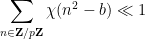
We will also need another easy case of the Weil bound to handle some other portions of (2):
Lemma 3 (Easy Weil bound) Let. Then
Proof: As 


 . As is
  on the quadratic residues and
  on the non-residues, it now suffices to show that
 , the left-hand side becomes
  , and the claim follows.
While the basic strategy of Heath-Brown’s argument is relatively straightforward, implementing it requires a large amount of computation to control both main terms and error terms. I experimented for a while with rearranging the argument to try to reduce the amount of computation; I did not fully succeed in arriving at a satisfactorily minimal amount of superfluous calculation, but I was able to at least reduce this amount a bit, mostly by replacing a combinatorial sieve with a Selberg-type sieve (which was not needed to be positive, so I dispensed with the squaring aspect of the Selberg sieve to simplify the calculations a little further; also for minor reasons it was convenient to retain a tiny portion of the combinatorial sieve to eliminate extremely small primes). Also some modest reductions in complexity can be obtained by using the second von Mangoldt function 

The Poincaré upper half-plane 


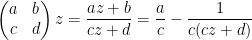
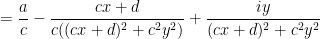
via fractional linear transformations:

Here and in the rest of the post we will abuse notation by identifying elements 


As the action of 


(using Cartesian coordinates 

the volume measure 

and the Laplace-Beltrami operator, which can be computed to be 


The Gauss curvature of the Poincaré half-plane can be computed to be the constant 


One can inject arithmetic into this geometric structure by passing from the Lie group
or congruence subgroups such as
for natural number 
These are discrete subgroups of

There are many further discrete subgroups of
Any discrete subgroup 


For instance, a fundamental domain for 


![\displaystyle [\hbox{PSL}_2({\bf Z}) : \Gamma_0(q)] = q \prod_{p|q} (1 + \frac{1}{p}) = q^{1+o(1)}](https://s0.wp.com/latex.php?latex=%5Cdisplaystyle++%5B%5Chbox%7BPSL%7D_2%28%7B%5Cbf+Z%7D%29+%3A+%5CGamma_0%28q%29%5D+%3D+q+%5Cprod_%7Bp%7Cq%7D+%281+%2B+%5Cfrac%7B1%7D%7Bp%7D%29+%3D+q%5E%7B1%2Bo%281%29%7D+&bg=ffffff&fg=000000&s=0&c=20201002)
copies of a fundamental domain for
While fundamental domains can be a convenient choice of coordinates to work with for some computations (as well as for drawing appropriate pictures), it is geometrically more natural to avoid working explicitly on such domains, and instead work directly on the quotient spaces 


An important way to create a ![{P_\Gamma[f]: {\mathbf H} \rightarrow {\bf C}}](https://s0.wp.com/latex.php?latex=%7BP_%5CGamma%5Bf%5D%3A+%7B%5Cmathbf+H%7D+%5Crightarrow+%7B%5Cbf+C%7D%7D&bg=ffffff&fg=000000&s=0&c=20201002)
 = \sum_{\gamma \in \Gamma} f(\gamma z),](https://s0.wp.com/latex.php?latex=%5Cdisplaystyle++P_%7B%5CGamma%7D%5Bf%5D%28z%29+%3D+%5Csum_%7B%5Cgamma+%5Cin+%5CGamma%7D+f%28%5Cgamma+z%29%2C&bg=ffffff&fg=000000&s=0&c=20201002)
which is clearly 

![{P_{\Gamma_\infty \backslash \Gamma}[f]: {\mathbf H} \rightarrow {\bf C}}](https://s0.wp.com/latex.php?latex=%7BP_%7B%5CGamma_%5Cinfty+%5Cbackslash+%5CGamma%7D%5Bf%5D%3A+%7B%5Cmathbf+H%7D+%5Crightarrow+%7B%5Cbf+C%7D%7D&bg=ffffff&fg=000000&s=0&c=20201002)
 = \sum_{\gamma \in \hbox{Fund}(\Gamma_\infty \backslash \Gamma)} f(\gamma z)](https://s0.wp.com/latex.php?latex=%5Cdisplaystyle++P_%7B%5CGamma_%5Cinfty+%5Cbackslash+%5CGamma%7D%5Bf%5D%28z%29+%3D+%5Csum_%7B%5Cgamma+%5Cin+%5Chbox%7BFund%7D%28%5CGamma_%5Cinfty+%5Cbackslash+%5CGamma%29%7D+f%28%5Cgamma+z%29&bg=ffffff&fg=000000&s=0&c=20201002)
where 


![{P_{\Gamma_\infty \backslash \Gamma}[f]}](https://s0.wp.com/latex.php?latex=%7BP_%7B%5CGamma_%5Cinfty+%5Cbackslash+%5CGamma%7D%5Bf%5D%7D&bg=ffffff&fg=000000&s=0&c=20201002)
For future reference we record the basic but fundamental unfolding identities
![\displaystyle \int_{\Gamma \backslash {\mathbf H}} P_\Gamma[f] g\ d\mu_{\Gamma \backslash {\mathbf H}} = \int_{\mathbf H} f g\ d\mu_{\mathbf H} \ \ \ \ \ (5)](https://s0.wp.com/latex.php?latex=%5Cdisplaystyle++%5Cint_%7B%5CGamma+%5Cbackslash+%7B%5Cmathbf+H%7D%7D+P_%5CGamma%5Bf%5D+g%5C+d%5Cmu_%7B%5CGamma+%5Cbackslash+%7B%5Cmathbf+H%7D%7D+%3D+%5Cint_%7B%5Cmathbf+H%7D+f+g%5C+d%5Cmu_%7B%5Cmathbf+H%7D+%5C+%5C+%5C+%5C+%5C+%285%29&bg=ffffff&fg=000000&s=0&c=20201002)
for any function 
![\displaystyle \int_{\Gamma \backslash {\mathbf H}} P_{\Gamma_\infty \backslash \Gamma}[f] g\ d\mu_{\Gamma \backslash {\mathbf H}} = \int_{\Gamma_\infty \backslash {\mathbf H}} f g\ d\mu_{\Gamma_\infty \backslash {\mathbf H}} \ \ \ \ \ (6)](https://s0.wp.com/latex.php?latex=%5Cdisplaystyle++%5Cint_%7B%5CGamma+%5Cbackslash+%7B%5Cmathbf+H%7D%7D+P_%7B%5CGamma_%5Cinfty+%5Cbackslash+%5CGamma%7D%5Bf%5D+g%5C+d%5Cmu_%7B%5CGamma+%5Cbackslash+%7B%5Cmathbf+H%7D%7D+%3D+%5Cint_%7B%5CGamma_%5Cinfty+%5Cbackslash+%7B%5Cmathbf+H%7D%7D+f+g%5C+d%5Cmu_%7B%5CGamma_%5Cinfty+%5Cbackslash+%7B%5Cmathbf+H%7D%7D+%5C+%5C+%5C+%5C+%5C+%286%29&bg=ffffff&fg=000000&s=0&c=20201002)
whenever 
When computing various statistics of a Poincaré series ![{P_\Gamma[f]}](https://s0.wp.com/latex.php?latex=%7BP_%5CGamma%5Bf%5D%7D&bg=ffffff&fg=000000&s=0&c=20201002)
}](https://s0.wp.com/latex.php?latex=%7BP_%5CGamma%5Bf%5D%28z%29%7D&bg=ffffff&fg=000000&s=0&c=20201002)


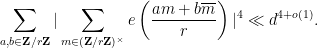
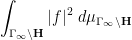
![{\int_{\Gamma \backslash {\mathbf H}} |P_\Gamma[f]|^2\ d\mu}](https://s0.wp.com/latex.php?latex=%7B%5Cint_%7B%5CGamma+%5Cbackslash+%7B%5Cmathbf+H%7D%7D+%7CP_%5CGamma%5Bf%5D%7C%5E2%5C+d%5Cmu%7D&bg=ffffff&fg=000000&s=0&c=20201002)
The first example we will give concerns the problem of estimating the sum
where 


which is basically a sum over the full modular group 
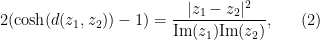
This sum is not exactly the same as (8), but will be a little easier to handle, and it is plausible that the methods used to handle this sum can be modified to handle (8). Observe from (2) and some calculation that the distance between 
and so one can express the above sum as

(the factor of 

}](https://s0.wp.com/latex.php?latex=%7BP_%5CGamma%5Bf%5D%28i%29%7D&bg=ffffff&fg=000000&s=0&c=20201002)

The second example concerns the relative

of the sum (7). Note from multiplicativity that (7) can be written as 

As with (7), we may expand (10) as
At first glance this does not look like a sum over a modular group, but one can manipulate this expression into such a form in one of two (closely related) ways. First, observe that any factorisation 


and one the modular group 


which (up to a harmless sign) is exactly the representation 

Note that 


Sums involving subgroups of the full modular group, such as 

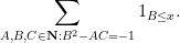
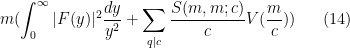
The third and final example concerns averages of Kloosterman sums
where 


![\displaystyle \int_{\Gamma_0(q) \backslash {\mathbf H}} |P_{\Gamma_\infty \backslash \Gamma_0(q)}[f]|^2\ d\mu_{\Gamma \backslash {\mathbf H}} \ \ \ \ \ (13)](https://s0.wp.com/latex.php?latex=%5Cdisplaystyle++%5Cint_%7B%5CGamma_0%28q%29+%5Cbackslash+%7B%5Cmathbf+H%7D%7D+%7CP_%7B%5CGamma_%5Cinfty+%5Cbackslash+%5CGamma_0%28q%29%7D%5Bf%5D%7C%5E2%5C+d%5Cmu_%7B%5CGamma+%5Cbackslash+%7B%5Cmathbf+H%7D%7D+%5C+%5C+%5C+%5C+%5C+%2813%29&bg=ffffff&fg=000000&s=0&c=20201002)
where

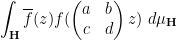
for some integer 
![\displaystyle \int_{\Gamma_\infty \backslash {\mathbf H}} \overline{f} P_{\Gamma_\infty \backslash \Gamma_0(q)}[f]\ d\mu_{\Gamma_\infty \backslash {\mathbf H}}.](https://s0.wp.com/latex.php?latex=%5Cdisplaystyle++%5Cint_%7B%5CGamma_%5Cinfty+%5Cbackslash+%7B%5Cmathbf+H%7D%7D+%5Coverline%7Bf%7D+P_%7B%5CGamma_%5Cinfty+%5Cbackslash+%5CGamma_0%28q%29%7D%5Bf%5D%5C+d%5Cmu_%7B%5CGamma_%5Cinfty+%5Cbackslash+%7B%5Cmathbf+H%7D%7D.&bg=ffffff&fg=000000&s=0&c=20201002)
To compute this, we use the double coset decomposition
where for each 

![{[1,c]}](https://s0.wp.com/latex.php?latex=%7B%5B1%2Cc%5D%7D&bg=ffffff&fg=000000&s=0&c=20201002)
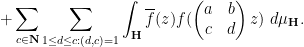
![\displaystyle P_{\Gamma_\infty \backslash \Gamma_0(q)}[f] = f + \sum_{c \in {\mathbf N}: q|c} \sum_{1 \leq d \leq c: (d,c)=1} P_{\Gamma_\infty}[ f( \begin{pmatrix} a & b \\ c & d \end{pmatrix} \cdot ) ]](https://s0.wp.com/latex.php?latex=%5Cdisplaystyle++P_%7B%5CGamma_%5Cinfty+%5Cbackslash+%5CGamma_0%28q%29%7D%5Bf%5D+%3D+f+%2B+%5Csum_%7Bc+%5Cin+%7B%5Cmathbf+N%7D%3A+q%7Cc%7D+%5Csum_%7B1+%5Cleq+d+%5Cleq+c%3A+%28d%2Cc%29%3D1%7D+P_%7B%5CGamma_%5Cinfty%7D%5B+f%28+%5Cbegin%7Bpmatrix%7D+a+%26+b+%5C%5C+c+%26+d+%5Cend%7Bpmatrix%7D+%5Ccdot+%29+%5D&bg=ffffff&fg=000000&s=0&c=20201002)
and so from further use of the unfolding formula (5) we may expand (13) as
The first integral is just 
so we can write
as


which on shifting 


and then on scaling 

Note that as 
where

is a certain integral involving 


Traditionally, automorphic forms have been analysed using the spectral theory of the Laplace-Beltrami operator 


for 


However, as discussed in this previous post, the spectral theory of an essentially self-adjoint operator such as 

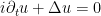


Actually it will be a bit more convenient to normalise the Laplacian by 

This equation somewhat resembles a “Klein-Gordon” type equation, except that the mass is imaginary! This would lead to pathological behaviour were it not for the negative curvature, which in principle creates a spectral gap of
The point is that the wave equation approach gives access to some nice PDE techniques, such as energy methods, Sobolev inequalities and finite speed of propagation, which are somewhat submerged in the spectral framework. The wave equation also interacts well with Poincaré series; if for instance ![{P_{\Gamma_\infty \backslash \Gamma}[u]}](https://s0.wp.com/latex.php?latex=%7BP_%7B%5CGamma_%5Cinfty+%5Cbackslash+%5CGamma%7D%5Bu%5D%7D&bg=ffffff&fg=000000&s=0&c=20201002)
![{P_{\Gamma_\infty \backslash \Gamma}[F]}](https://s0.wp.com/latex.php?latex=%7BP_%7B%5CGamma_%5Cinfty+%5Cbackslash+%5CGamma%7D%5BF%5D%7D&bg=ffffff&fg=000000&s=0&c=20201002)
- Using the Weil bound on Kloosterman sums to derive Selberg’s 3/16 theorem on the least non-trivial eigenvalue for
- Conversely, showing that Selberg’s eigenvalue conjecture (improving Selberg’s
bound to the optimal
) implies an optimal bound on (smoothed) sums of Kloosterman sums; and
- Using the same bound to obtain pointwise bounds on Poincaré series similar to the ones discussed above. (Actually, the argument here does not use the wave equation, instead it just uses the Sobolev inequality.)
This post originated from an attempt to finally learn this part of analytic number theory properly, and to see if I could use a PDE-based perspective to understand it better. Ultimately, this is not that dramatic a depature from the standard approach to this subject, but I found it useful to think of things in this fashion, probably due to my existing background in PDE.
I thank Bill Duke and Ben Green for helpful discussions. My primary reference for this theory was Chapters 15, 16, and 21 of Iwaniec and Kowalski.
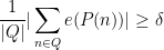
The equidistribution theorem asserts that if 


for any continuous (or equivalently, for any smooth) function 

for any non-zero integer 


One can then ask for more quantitative information about the decay of exponential sums of 


Lemma 1 (Geometric series formula, inverse form) Let
be an arithmetic progression of length at most
for some
, and let
be a linear polynomial for some
. If
for some
, then there exists a subprogression
of
such that
varies by at most
on
of length at most

Proof: By a linear change of variable we may assume that 


and so 

Thus, in order for a linear phase 
As is well known, this phenomenon generalises to higher order polynomials. To achieve this, we need two elementary additional lemmas. The first relates the exponential sums of 
Lemma 2 (Van der Corput lemma, inverse form) Let
be an arbitrary function such that
for some
integers
, there exists a subprogression
of


Proof: Squaring (1), we see that

We write 

where 


for
The second lemma (which we recycle from this previous blog post) is a variant of the equidistribution theorem.
Lemma 3 (Vinogradov lemma) Let
be an interval for some
be such that
for at least
values of
, for some
. Then either
or
or else there is a natural number
such that


Proof: We may assume that 


We take 

If 


By hypothesis, 


We conclude that for fixed 

![{[n, n + \frac{1}{10 |\kappa|}]}](https://s0.wp.com/latex.php?latex=%7B%5Bn%2C+n+%2B+%5Cfrac%7B1%7D%7B10+%7C%5Ckappa%7C%7D%5D%7D&bg=ffffff&fg=000000&s=0&c=20201002)


and the claim follows.
Now we can quickly obtain a higher degree version of Lemma 1:
Proposition 4 (Weyl exponential sum estimate, inverse form) Let
be a polynomial of some degree at most
. If
for some
such that
Proof: We induct on 


By rescaling we may assume ![{Q \subset [0,N] \cap {\bf Z}}](https://s0.wp.com/latex.php?latex=%7BQ+%5Csubset+%5B0%2CN%5D+%5Ccap+%7B%5Cbf+Z%7D%7D&bg=ffffff&fg=000000&s=0&c=20201002)
![{h \in [-N,N] \cap {\bf Z}}](https://s0.wp.com/latex.php?latex=%7Bh+%5Cin+%5B-N%2CN%5D+%5Ccap+%7B%5Cbf+Z%7D%7D&bg=ffffff&fg=000000&s=0&c=20201002)

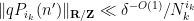
for some interval ![{I_h \subset [0,N] \cap {\bf Z}}](https://s0.wp.com/latex.php?latex=%7BI_h+%5Csubset+%5B0%2CN%5D+%5Ccap+%7B%5Cbf+Z%7D%7D&bg=ffffff&fg=000000&s=0&c=20201002)


![{[-\delta^{-O(1)} N, \delta^{-O(1)} N] \cap {\bf Z}}](https://s0.wp.com/latex.php?latex=%7B%5B-%5Cdelta%5E%7B-O%281%29%7D+N%2C+%5Cdelta%5E%7B-O%281%29%7D+N%5D+%5Ccap+%7B%5Cbf+Z%7D%7D&bg=ffffff&fg=000000&s=0&c=20201002)


In the former case the claim is trivial (just take
We partition 
so by the pigeonhole principle, we have

for at least one such progression 


and hence by induction hypothesis we may find a subprogression 


This gives the following corollary (also given as Exercise 16 in this previous blog post):
Corollary 5 (Weyl exponential sum estimate, inverse form II) Let
. If
for some
such that
for all
.

One can obtain much better exponents here using Vinogradov’s mean value theorem; see Theorem 1.6 this paper of Wooley. (Thanks to Mariusz Mirek for this reference.) However, this weaker result already suffices for many applications, and does not need any result as deep as the mean value theorem.
Proof: To simplify notation we allow implied constants to depend on 

Applying Proposition 4, we can find a natural number 


![{I' \subset [0,N] \cap {\bf Z}}](https://s0.wp.com/latex.php?latex=%7BI%27+%5Csubset+%5B0%2CN%5D+%5Ccap+%7B%5Cbf+Z%7D%7D&bg=ffffff&fg=000000&s=0&c=20201002)


For future reference we also record a higher degree version of the Vinogradov lemma.
Lemma 6 (Polynomial Vinogradov lemma) Let
such that
for at least
or else there is a natural number
for all


Proof: We induct on 

For each ![{h \in [-2N,2N] \cap {\bf Z}}](https://s0.wp.com/latex.php?latex=%7Bh+%5Cin+%5B-2N%2C2N%5D+%5Ccap+%7B%5Cbf+Z%7D%7D&bg=ffffff&fg=000000&s=0&c=20201002)

![{n \in [-N,N] \cap {\bf Z}}](https://s0.wp.com/latex.php?latex=%7Bn+%5Cin+%5B-N%2CN%5D+%5Ccap+%7B%5Cbf+Z%7D%7D&bg=ffffff&fg=000000&s=0&c=20201002)

![{\sum_{h \in [-2N,2N] \cap {\bf Z}} N_h \gg \delta^2 N^2}](https://s0.wp.com/latex.php?latex=%7B%5Csum_%7Bh+%5Cin+%5B-2N%2C2N%5D+%5Ccap+%7B%5Cbf+Z%7D%7D+N_h+%5Cgg+%5Cdelta%5E2+N%5E2%7D&bg=ffffff&fg=000000&s=0&c=20201002)


for 


Since 
for

We can again assume it is the latter that holds. This implies that 

for
The above results also extend to higher dimensions. Here is the higher dimensional version of Proposition 4:
Proposition 7 (Multidimensional Weyl exponential sum estimate, inverse form) Let
and
, and let
be arithmetic progressions of length at most
for each
. Let
be a polynomial of degrees at most
in each of the
variables
separately. If
for some
of
with
for each
.
A much more general statement, in which the polynomial phase 
Proof: We induct on 


By a linear change of variables, we may assume that ![{Q_i \subset [0,N_i] \cap {\bf Z}}](https://s0.wp.com/latex.php?latex=%7BQ_i+%5Csubset+%5B0%2CN_i%5D+%5Ccap+%7B%5Cbf+Z%7D%7D&bg=ffffff&fg=000000&s=0&c=20201002)
We write 

and the claim then follows from the induction hypothesis. Thus we may assume that 

By the triangle inequality, we have
The inner sum is 

for some polynomials 


for 

for all 

where 


Applying Lemma 6 in the 


for all 

whenever 


An inspection of the proof of the above result (or alternatively, by combining the above result again with many applications of Lemma 6) reveals the following general form of Proposition 4, which was posed as Exercise 17 in this previous blog post, but had a slight misprint in it (it did not properly treat the possibility that some of the 
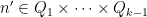
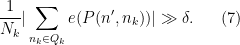
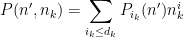
Proposition 8 (Multidimensional Weyl exponential sum estimate, inverse form, II) Let
be a discrete interval for some
. Let
be a polynomial in
for some
. If
for some
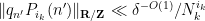
, or else there is a natural number
such that


 for
for Again, the factor of 


![{\sum_{n_1 \in \{0,1\}} \sum_{n_2 \in [1,N] \cap {\bf Z}} e( \alpha n_1 n_2)}](https://s0.wp.com/latex.php?latex=%7B%5Csum_%7Bn_1+%5Cin+%5C%7B0%2C1%5C%7D%7D+%5Csum_%7Bn_2+%5Cin+%5B1%2CN%5D+%5Ccap+%7B%5Cbf+Z%7D%7D+e%28+%5Calpha+n_1+n_2%29%7D&bg=ffffff&fg=000000&s=0&c=20201002)
Chantal David, Andrew Granville, Emmanuel Kowalski, Phillipe Michel, Kannan Soundararajan, and I are running a program at MSRI in the Spring of 2017 (more precisely, from Jan 17, 2017 to May 26, 2017) in the area of analytic number theory, with the intention to bringing together many of the leading experts in all aspects of the subject and to present recent work on the many active areas of the subject (the discussion on previous blog posts here have mostly focused on advances in the study of the distribution of the prime numbers, but there have been many other notable recent developments too, such as refinements of the circle method, a deeper understanding of the asymptotics of bounded multiplicative functions and of the “pretentious” approach to analytic number theory, more “analysis-friendly” formulations of the theorems of Deligne and others involving trace functions over fields, and new subconvexity theorems for automorphic forms, to name a few). Like any other semester MSRI program, there will be a number of workshops, seminars, and similar activities taking place while the members are in residence. I’m personally looking forward to the program, which should be occurring in the midst of a particularly productive time for the subject. Needless to say, I (and the rest of the organising committee) plan to be present for most of the program.
Applications for Postdoctoral Fellowships, Research Memberships, and Research Professorships for this program (and for other MSRI programs in this time period, namely the companion program in Harmonic Analysis and the Fall program in Geometric Group Theory, as well as the complementary program in all other areas of mathematics) have just opened up today. Applications are open to everyone (until they close on Dec 1), but require supporting documentation, such as a CV, statement of purpose, and letters of recommendation from other mathematicians; see the application page for more details.

Recent Comments