
You are currently browsing the category archive for the ‘tricks’ category.
A common task in analysis is to obtain bounds on sums


 is some simple region (such as an interval) in one or more dimensions, and
  is an explicit (and elementary) non-negative expression involving one or more variables (such as
  or
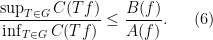
or  , and possibly also some additional parameters. Often, one would be content with an order of magnitude upper bound such as

 (or
(or  or
or  ) to denote the bound
  for some constant
  ; sometimes one wishes to also obtain the matching lower bound, thus obtaining
 is synonymous with
  . Finally, one may wish to obtain a more precise bound, such as
 is a quantity that goes to zero as the parameters of the problem go to infinity (or some other limit). (For a deeper dive into asymptotic notation in general, see this previous blog post.)
Here are some typical examples of such estimation problems, drawn from recent questions on MathOverflow:
- (i) (From this question) If
and
, is the expression
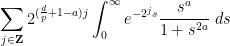
finite? - (ii) (From this question) If
, how can one show that
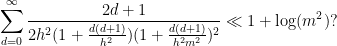
- (iii) (From this question) Can one show that
asfor an explicit constant
, and what is this constant?

Compared to other estimation tasks, such as that of controlling oscillatory integrals, exponential sums, singular integrals, or expressions involving one or more unknown functions (that are only known to lie in some function spaces, such as an 
Somewhat in the spirit of this previous post on analysis problem solving strategies, I am going to try here to collect some general principles and techniques that I have found useful for these sorts of problems. As with the previous post, I hope this will be something of a living document, and encourage others to add their own tips or suggestions in the comments.
The “epsilon-delta” nature of analysis can be daunting and unintuitive to students, as the heavy reliance on inequalities rather than equalities. But it occurred to me recently that one might be able to leverage the intuition one already has from “deals” – of the type one often sees advertised by corporations – to get at least some informal understanding of these concepts.
Take for instance the concept of an upper bound 


| Currency | We buy at | We sell at |
 |  |  |
 | – |  |
 |  | |
 | – |  |
Someone with an eye for spotting “deals” might now realize that one can actually buy 


Asymptotic estimates such as 

When it comes to the basic analysis concepts of convergence and continuity, one can similarly view these concepts as various economic transactions involving the buying and selling of accuracy. One could for instance imagine the following hypothetical range of products in which one would need to spend more money to obtain higher accuracy to measure weight in grams:
| Object | Accuracy | Price |
| Low-end kitchen scale |  gram gram |  |
| High-end bathroom scale |  grams grams |  |
| Low-end lab scale |  grams grams |  |
| High-end lab scale |  grams grams |  |
The concept of convergence 


| Status | Accuracy benefit | Eligibility |
| Basic status |  |  |
| Bronze status |  |  |
| Silver status |  |  |
| Gold status |  |  |
 | | |
With this conceptual model, convergence means that any status level of accuracy can be unlocked if one’s number
In a similar vein, continuity becomes analogous to a conversion program, in which accuracy benefits from one company can be traded in for new accuracy benefits in another company. For instance, the continuity of the function 

| Accuracy benefit of to trade in | Accuracy benefit of  obtained obtained |
 |  |
 |  |
 |  |
| | |
Again, the point is that one can purchase any desired level of accuracy of
At present, the above conversion chart is only available at the single location 

In a similar vein, differentiability can be viewed as a deal in which one can trade in accuracy of the input for approximately linear behavior of the output; to oversimplify slightly, smoothness can similarly be viewed as a deal in which one trades in accuracy of the input for high-accuracy polynomial approximability of the output. Measurability of a set or function can be viewed as a deal in which one trades in a level of resolution for an accurate approximation of that set or function at the given resolution. And so forth.
Perhaps readers can propose some other examples of mathematical concepts being re-interpreted as some sort of economic transaction?
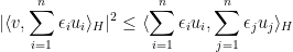
In this previous blog post I noted the following easy application of Cauchy-Schwarz:
Lemma 1 (Van der Corput inequality) Letbe unit vectors in a Hilbert space
. Then

Proof: The left-hand side may be written as 


As a corollary, correlation becomes transitive in a statistical sense (even though it is not transitive in an absolute sense):
Corollary 2 (Statistical transitivity of correlation) Letfor all
and some
. Then we have
for at least
of the pairs
.
Proof: From the lemma, we have
 with
with  is at most , and all the remaining summands are at most
  , giving the claim.
One drawback with this corollary is that it does not tell us which pairs 


While working on an ongoing research project, I recently found that there is a very simple way to get around the latter problem by exploiting the tensor power trick:
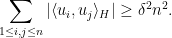
Corollary 3 (Simultaneous statistical transitivity of correlation) Letbe unit vectors in a Hilbert space for
such that
for all
. Then there are at least
pairs
. In particular (by Cauchy-Schwarz) we have
for all
.
Proof: Apply Corollary 2 to the unit vectors 


It is surprisingly difficult to obtain even a qualitative version of the above conclusion (namely, if 


 is the orthogonal projection to the complement of . This implies a Gram matrix inequality
  where
where  denotes the claim that
  is positive semi-definite. By the Schur product theorem, we conclude that
 ,
, 
A separate application of tensor powers to amplify correlations was also noted in this previous blog post giving a cheap version of the Kabatjanskii-Levenstein bound, but this seems to not be directly related to this current application.
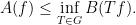
In one of the earliest posts on this blog, I talked about the ability to “arbitrage” a disparity of symmetry in an inequality, and in particular to “amplify” such an inequality into a stronger one. (The principle can apply to other mathematical statements than inequalities, with the “hypothesis” and “conclusion” of that statement generally playing the role of the “right-hand side” and “left-hand side” of an inequality, but for sake of discussion I will restrict attention here to inequalities.) One can formalise this principle as follows. Many inequalities in analysis can be expressed in the form

for all 


for all symmetries 

Suppose we know that the inequality (1) holds for all 
In particular, it is often the case that there is a way to send 


of (1). Note that these amplified inequalities will now be 
and in particular (if 


If neither
though now this inequality is not obviously stronger than the original inequality (1) (for instance it could well be trivial). In some cases one can also average over
As discussed in the previous post, this use of amplification gives rise to a general principle about inequalities: the most efficient inequalities are those in which the left-hand side and right-hand side enjoy the same symmetries. It is certainly possible to have true inequalities that have an imbalance of symmetry, but as shown above, such inequalities can always be amplified to more efficient and more symmetric inequalities. In the case when limits such as 

One often tries to prove inequalities (1) by directly chaining together simpler inequalities. For instance, one might attempt to prove (1) by by first bounding 

A variant of the above principle then asserts that when proving inequalities by such direct methods, one should, whenever possible, try to maintain the symmetries that are present in both sides of the inequality. Why? Well, suppose that we ignored this principle and tried to prove (1) by establishing (4) for some 
and also amplify the second half 

and hence (4) amplifies to

Let’s say for sake of argument that all the quantities involved here are positive numbers (which is often the case in analysis). Then we see in particular that
Informally, (6) asserts that in order for the strategy (4) used to prove (1) to work, the extent to which

(assuming that the appropriate limit 
Here are some simple (but somewhat contrived) examples to illustrate these points. Suppose one wishes to prove the inequality
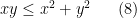
for all 


to conclude that
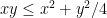
and then use the obvious inequality 


of (8) (that is to say, the arithmetic mean-geometric mean inequality). Try it!
Similarly, consider the task of proving the triangle inequality

for complex numbers 
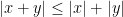

and then use the real triangle inequality to obtain

and

and then finally use the inequalities


but when one puts this all together at the end of the day, one loses a factor of two:

One can “blame” this loss on the fact that while the original inequality (9) was invariant with respect to phase rotation 

Here is a slight variant of the above example. Suppose that you had just learned in class to prove the triangle inequality
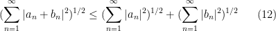
for (say) real square-summable sequences 


for doubly infinite square-summable sequences 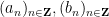


for any 

Note that the principle of preserving symmetry only applies to direct approaches to proving inequalities such as (1). There is a complementary approach, discussed for instance in this previous post, which is to spend the symmetry to place the variable 


As a simple example of this, let us revisit the complex triangle inequality (9). As already noted, both sides of this inequality are invariant with respect to the phase rotation symmetry 


and the triangle inequality (9) is now an immediate consequence of (10), (11). (But note that if one had unwisely spent the symmetry to normalise, say,
A few days ago, I was talking with Ed Dunne, who is currently the Executive Editor of Mathematical Reviews (and in particular with its online incarnation at MathSciNet). At the time, I was mentioning how laborious it was for me to create a BibTeX file for dozens of references by using MathSciNet to locate each reference separately, and to export each one to BibTeX format. He then informed me that underneath to every MathSciNet reference there was a little link to add the reference to a Clipboard, and then one could export the entire Clipboard at once to whatever format one wished. In retrospect, this was a functionality of the site that had always been visible, but I had never bothered to explore it, and now I can populate a BibTeX file much more quickly.
This made me realise that perhaps there are many other useful features of popular mathematical tools out there that only a few users actually know about, so I wanted to create a blog post to encourage readers to post their own favorite tools, or features of tools, that are out there, often in plain sight, but not always widely known. Here are a few that I was able to recall from my own workflow (though for some of them it took quite a while to consciously remember, since I have been so used to them for so long!):
- TeX for Gmail. A Chrome plugin that lets one write TeX symbols in emails sent through Gmail (by writing the LaTeX code and pressing a hotkey, usually F8).
- Boomerang for Gmail. Another Chrome plugin for Gmail, which does two main things. Firstly, it can “boomerang” away an email from your inbox to return at some specified later date (e.g. one week from today). I found this useful to declutter my inbox regarding mail that I needed to act on in the future, but was unable to deal with at present due to travel, or because I was waiting for some other piece of data to arrive first. Secondly, it can send out email with some specified delay (e.g. by tomorrow morning), giving one time to cancel the email if necessary. (Thanks to Julia Wolf for telling me about Boomerang!)
- Which just reminds me, the Undo Send feature on Gmail has saved me from embarrassment a few times (but one has to set it up first; it delays one’s emails by a short period, such as 30 seconds, during which time it is possible to undo the email).
- LaTeX rendering in Inkscape. I used to use plain text to write mathematical formulae in my images, which always looked terrible. It took me years to realise that Inkscape had the functionality to compile LaTeX within it.
- Bookmarks in TeXnicCenter. I probably only use a tiny fraction of the functionality that TeXnicCenter offers, but one little feature I quite like is the ability to bookmark a portion of the TeX file (e.g. the bibliography at the end, or the place one is currently editing) with one hot-key (Ctrl-F2) and then one can cycle quickly between one bookmarked location and another with some further hot-keys (F2 and shift-F2).
- Actually, there are a number of Windows keyboard shortcuts that are worth experimenting with (and similarly for Mac or Linux systems of course).
- Detexify has been the quickest way for me to locate the TeX code for a symbol that I couldn’t quite remember (or when hunting for a new symbol that would roughly be shaped like something I had in mind).
- For writing LaTeX on my blog, I use Luca Trevisan’s LaTeX to WordPress Python script (together with a little batch file I wrote to actually run the python script).
- Using the camera on my phone to record a blackboard computation or a slide (or the wifi password at a conference centre, or any other piece of information that is written or displayed really). If the phone is set up properly this can be far quicker than writing it down with pen and paper. (I guess this particular trick is now quite widely used, but I still see people surprised when someone else uses a phone instead of a pen to record things.)
- Using my online calendar not only to record scheduled future appointments, but also to block out time to do specific tasks (e.g. reserve 2-3pm at Tuesday to read paper X, or do errand Y). I have found I am able to get a much larger fraction of my “to do” list done on days in which I had previously blocked out such specific chunks of time, as opposed to days in which I had left several hours unscheduled (though sometimes those hours were also very useful for finding surprising new things to do that I had not anticipated). (I learned of this little trick online somewhere, but I have long since lost the original reference.)
Anyway, I would very much like to hear what other little tools or features other readers have found useful in their work.
This is going to be a somewhat experimental post. In class, I mentioned that when solving the type of homework problems encountered in a graduate real analysis course, there are really only about a dozen or so basic tricks and techniques that are used over and over again. But I had not thought to actually try to make these tricks explicit, so I am going to try to compile here a list of some of these techniques here. But this list is going to be far from exhaustive; perhaps if other recent students of real analysis would like to share their own methods, then I encourage you to do so in the comments (even – or especially – if the techniques are somewhat vague and general in nature).
(See also the Tricki for some general mathematical problem solving tips. Once this page matures somewhat, I might migrate it to the Tricki.)
Note: the tricks occur here in no particular order, reflecting the stream-of-consciousness way in which they were arrived at. Indeed, this list will be extended on occasion whenever I find another trick that can be added to this list.
This is a technical post inspired by separate conversations with Jim Colliander and with Soonsik Kwon on the relationship between two techniques used to control non-radiating solutions to dispersive nonlinear equations, namely the “double Duhamel trick” and the “in/out decomposition”. See for instance these lecture notes of Killip and Visan for a survey of these two techniques and other related methods in the subject. (I should caution that this post is likely to be unintelligible to anyone not already working in this area.)
For sake of discussion we shall focus on solutions to a nonlinear Schrödinger equation

and we will not concern ourselves with the specific regularity of the solution 

Solutions to this equation enjoy the forward Duhamel formula
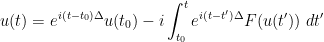
for times 


for all times 


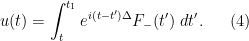
The situation is reversed when one turns to the global theory, and looks at the asymptotic behaviour of a solution as one approaches a limiting time
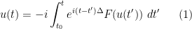

where 
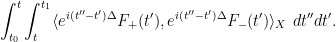
A key task is then to somehow combine the forward representation (1) and the backward representation (2) to obtain new information on 


where 

Typically, one already has (or is willing to assume as a bootstrap hypothesis) control on 


One can use some classical functional analysis to clarify this situation. By the closed graph theorem, the above task is (morally, at least) equivalent to establishing an a priori bound of the form

for all reasonable

for all reasonable 


The dispersive nature of the linear Schrödinger equation often causes 

Unfortunately it appears that estimates of the form (6) fail in low dimensions (for the type of norms 


![{\| e^{i(\cdot-t)\Delta} u_+\|_{N^*([t_0,t])}}](https://s0.wp.com/latex.php?latex=%7B%5C%7C+e%5E%7Bi%28%5Ccdot-t%29%5CDelta%7D+u_%2B%5C%7C_%7BN%5E%2A%28%5Bt_0%2Ct%5D%29%7D%7D&bg=ffffff&fg=000000&s=0&c=20201002)

![{\| e^{i(\cdot-t)\Delta} u_-\|_{N^*([t,t_1])}}](https://s0.wp.com/latex.php?latex=%7B%5C%7C+e%5E%7Bi%28%5Ccdot-t%29%5CDelta%7D+u_-%5C%7C_%7BN%5E%2A%28%5Bt%2Ct_1%5D%29%7D%7D&bg=ffffff&fg=000000&s=0&c=20201002)
So one can dualise the task of proving (5) as that of obtaining a decomposition of an arbitrary initial state 

The in/out decomposition is a linear one, but the Hahn-Banach argument gives no reason why the decomposition needs to be linear. (Note that other well-known decompositions in analysis, such as the Fefferman-Stein decomposition of BMO, are necessarily nonlinear, a fact which is ultimately equivalent to the non-complemented nature of a certain subspace of a Banach space; see these lecture notes of mine and this old blog post for some discussion.) So one could imagine a sophisticated nonlinear decomposition as a general substitute for the in/out decomposition. See for instance this paper of Bourgain and Brezis for some of the subtleties of decomposition even in very classical function spaces such as 
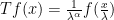
In this post I would like to make some technical notes on a standard reduction used in the (Euclidean, maximal) Kakeya problem, known as the two ends reduction. This reduction (which takes advantage of the approximate scale-invariance of the Kakeya problem) was introduced by Wolff, and has since been used many times, both for the Kakeya problem and in other similar problems (e.g. by Jim Wright and myself to study curved Radon-like transforms). I was asked about it recently, so I thought I would describe the trick here. As an application I give a proof of the 
From Tim Gowers’ blog comes the announcement that the Tricki – a wiki for various tricks and strategies for proving mathematical results – is now live. (My own articles for the Tricki are also on this blog; also Ben Green has written up an article on using finite fields to prove results about infinite fields which is loosely based on my own post on the topic, which is in turn based on an article of Serre.) It seems to already be growing at a reasonable rate, with many contributors.
Today I’d like to discuss (in the Tricks Wiki format) a fundamental trick in “soft” analysis, sometimes known as the “limiting argument” or “epsilon regularisation argument”.
Title: Give yourself an epsilon of room.
Quick description: You want to prove some statement 


One can of course play a similar game when proving a statement 


General discussion: Here are some typical examples of a target statement 
|
|
 |
 |
 |
 |
 |
 for some for some  independent of independent of |
 is finite is finite |
 is bounded uniformly in is bounded uniformly in |
 for all for all  (i.e. maximises f) (i.e. maximises f) |
 for all (i.e. nearly maximises f) for all (i.e. nearly maximises f) |
 converges as converges as  |
 fluctuates by at most o(1) for sufficiently large n fluctuates by at most o(1) for sufficiently large n |
 is a measurable function is a measurable function |
 is a measurable function converging pointwise to is a measurable function converging pointwise to |
| is a continuous function |
is an equicontinuous family of functions converging pointwise to OR is continuous and converges (locally) uniformly to |
The event  holds almost surely holds almost surely |
The event  holds with probability 1-o(1) holds with probability 1-o(1) |
The statement  holds for almost every x holds for almost every x |
The statement  holds for x outside of a set of measure o(1) holds for x outside of a set of measure o(1) |
Of course, to justify the convergence of 
It is also necessary in many cases that the control 
By giving oneself an epsilon of room, one can evade a lot of familiar issues in soft analysis. For instance, by replacing “rough”, “infinite-complexity”, “continuous”, “global”, or otherwise “infinitary” objects 

To summarise: one can view the epsilon regularisation argument as a “loan” in which one borrows an epsilon here and there in order to be able to ignore soft analysis difficulties, and can temporarily be able to utilise estimates which are non-uniform in epsilon, but at the end of the day one needs to “pay back” the loan by establishing a final “hard analysis” estimate which is uniform in epsilon (or whose error terms decay to zero as epsilon goes to zero).
A variant: It may seem that the epsilon regularisation trick is useless if one is already in “hard analysis” situations when all objects are already “finitary”, and all formal computations easily justified. However, there is an important variant of this trick which applies in this case: namely, instead of sending the epsilon parameter to zero, choose epsilon to be a sufficiently small (but not infinitesimally small) quantity, depending on other parameters in the problem, so that one can eventually neglect various error terms and to obtain a useful bound at the end of the day. (For instance, any result proven using the Szemerédi regularity lemma is likely to be of this type.) Since one is not sending epsilon to zero, not every term in the final bound needs to be uniform in epsilon, though for quantitative applications one still would like the dependencies on such parameters to be as favourable as possible.
Prerequisites: Graduate real analysis. (Actually, this isn’t so much a prerequisite as it is a corequisite: the limiting argument plays a central role in many fundamental results in real analysis.) Some examples also require some exposure to PDE.

Recent Comments