Exploring the toolkit of Jean Bourgain

I have uploaded to the arXiv my paper “Exploring the toolkit of Jean Bourgain“. This is one of a collection of papers to be published in the Bulletin of the American Mathematical Society describing aspects of the work of Jean Bourgain; other contributors to this collection include Keith Ball, Ciprian Demeter, and Carlos Kenig. Because the other contributors will be covering specific areas of Jean’s work in some detail, I decided to take a non-overlapping tack, and focus instead on some basic tools of Jean that he frequently used across many of the fields he contributed to. Jean had a surprising number of these “basic tools” that he wielded with great dexterity, and in this paper I focus on just a few of them:

• Reducing qualitative analysis results (e.g., convergence theorems or dimension bounds) to quantitative analysis estimates (e.g., variational inequalities or maximal function estimates).
• Using dyadic pigeonholing to locate good scales to work in or to apply truncations.
• Using random translations to amplify small sets (low density) into large sets (positive density).
• Combining large deviation inequalities with metric entropy bounds to control suprema of various random processes.

Each of these techniques is individually not too difficult to explain, and were certainly employed on occasion by various mathematicians prior to Bourgain’s work; but Jean had internalized them to the point where he would instinctively use them as soon as they became relevant to a given problem at hand. I illustrate this at the end of the paper with an exposition of one particular result of Jean, on the Erdős similarity problem, in which his main result (that any sum of three infinite sets of reals has the property that there exists a positive measure set that does not contain any homothetic copy of ) is basically proven by a sequential application of these tools (except for dyadic pigeonholing, which turns out not to be needed here).

I had initially intended to also cover some other basic tools in Jean’s toolkit, such as the uncertainty principle and the use of probabilistic decoupling, but was having trouble keeping the paper coherent with such a broad focus (certainly I could not identify a single paper of Jean’s that employed all of these tools at once). I hope though that the examples given in the paper gives some reasonable impression of Jean’s research style.

Quantitative bounds for critically bounded solutions to the Navier-Stokes equations

I’ve just uploaded to the arXiv my paper “Quantitative bounds for critically bounded solutions to the Navier-Stokes equations“, submitted to the proceedings of the Linde Hall Inaugural Math Symposium. (I unfortunately had to cancel my physical attendance at this symposium for personal reasons, but was still able to contribute to the proceedings.) In recent years I have been interested in working towards establishing the existence of classical solutions for the Navier-Stokes equations

that blow up in finite time, but this time for a change I took a look at the other side of the theory, namely the conditional regularity results for this equation. There are several such results that assert that if a certain norm of the solution stays bounded (or grows at a controlled rate), then the solution stays regular; taken in the contrapositive, they assert that if a solution blows up at a certain finite time , then certain norms of the solution must also go to infinity. Here are some examples (not an exhaustive list) of such blowup criteria:

• (Leray blowup criterion, 1934) If blows up at a finite time , and , then for an absolute constant .
• (Prodi–Serrin–Ladyzhenskaya blowup criterion, 1959-1967) If blows up at a finite time , and , then , where .
• (Beale-Kato-Majda blowup criterion, 1984) If blows up at a finite time , then , where is the vorticity.
• (Kato blowup criterion, 1984) If blows up at a finite time , then for some absolute constant .
• (Escauriaza-Seregin-Sverak blowup criterion, 2003) If blows up at a finite time , then .
• (Seregin blowup criterion, 2012) If blows up at a finite time , then .
• (Phuc blowup criterion, 2015) If blows up at a finite time , then for any .
• (Gallagher-Koch-Planchon blowup criterion, 2016) If blows up at a finite time , then for any .
• (Albritton blowup criterion, 2016) If blows up at a finite time , then for any .

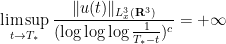
My current paper is most closely related to the Escauriaza-Seregin-Sverak blowup criterion, which was the first to show a critical (i.e., scale-invariant, or dimensionless) spatial norm, namely , had to become large. This result now has many proofs; for instance, many of the subsequent blowup criterion results imply the Escauriaza-Seregin-Sverak one as a special case, and there are also additional proofs by Gallagher-Koch-Planchon (building on ideas of Kenig-Koch), and by Dong-Du. However, all of these proofs rely on some form of a compactness argument: given a finite time blowup, one extracts some suitable family of rescaled solutions that converges in some weak sense to a limiting solution that has some additional good properties (such as almost periodicity modulo symmetries), which one can then rule out using additional qualitative tools, such as unique continuation and backwards uniqueness theorems for parabolic heat equations. In particular, all known proofs use some version of the backwards uniqueness theorem of Escauriaza, Seregin, and Sverak. Because of this reliance on compactness, the existing proofs of the Escauriaza-Seregin-Sverak blowup criterion are qualitative, in that they do not provide any quantitative information on how fast the norm will go to infinity (along a subsequence of times).

On the other hand, it is a general principle that qualitative arguments established using compactness methods ought to have quantitative analogues that replace the use of compactness by more complicated substitutes that give effective bounds; see for instance these previous blog posts for more discussion. I therefore was interested in trying to obtain a quantitative version of this blowup criterion that gave reasonably good effective bounds (in particular, my objective was to avoid truly enormous bounds such as tower-exponential or Ackermann function bounds, which often arise if one “naively” tries to make a compactness argument effective). In particular, I obtained the following triple-exponential quantitative regularity bounds:

Theorem 1 If is a classical solution to Navier-Stokes on with

 

for some , then

and

for and .

As a corollary, one can now improve the Escauriaza-Seregin-Sverak blowup criterion to

for some absolute constant , which to my knowledge is the first (very slightly) supercritical blowup criterion for Navier-Stokes in the literature.

The proof uses many of the same quantitative inputs as previous arguments, most notably the Carleman inequalities used to establish unique continuation and backwards uniqueness theorems for backwards heat equations, but also some additional techniques that make the quantitative bounds more efficient. The proof focuses initially on points of concentration of the solution, which we define as points where there is a frequency for which one has the bound

 

for a large absolute constant , where is a Littlewood-Paley projection to frequencies . (This can be compared with the upper bound of for the quantity on the left-hand side that follows from (1).) The factor of normalises the left-hand side of (2) to be dimensionless (i.e., critical). The main task is to show that the dimensionless quantity cannot get too large; in particular, we end up establishing a bound of the form

from which the above theorem ends up following from a routine adaptation of the local well-posedness and regularity theory for Navier-Stokes.

The strategy is to show that any concentration such as (2) when is large must force a significant component of the norm of to also show up at many other locations than , which eventually contradicts (1) if one can produce enough such regions of non-trivial norm. (This can be viewed as a quantitative variant of the “rigidity” theorems in some of the previous proofs of the Escauriaza-Seregin-Sverak theorem that rule out solutions that exhibit too much “compactness” or “almost periodicity” in the topology.) The chain of causality that leads from a concentration (2) at to significant norm at other regions of the time slice is somewhat involved (though simpler than the much more convoluted schemes I initially envisaged for this argument):

1. Firstly, by using Duhamel’s formula, one can show that a concentration (2) can only occur (with large) if there was also a preceding concentration

   

    

   at some slightly previous point in spacetime, with also close to (more precisely, we have , , and ). This can be viewed as a sort of contrapositive of a “local regularity theorem”, such as the ones established by Caffarelli, Kohn, and Nirenberg. A key point here is that the lower bound in the conclusion (3) is precisely the same as the lower bound in (2), so that this backwards propagation of concentration can be iterated.

2. Iterating the previous step, one can find a sequence of concentration points

   

    

   with the propagating backwards in time; by using estimates ultimately resulting from the dissipative term in the energy identity, one can extract such a sequence in which the increase geometrically with time, the are comparable (up to polynomial factors in ) to the natural frequency scale , and one has . Using the “epochs of regularity” theory that ultimately dates back to Leray, and tweaking the slightly, one can also place the times in intervals (of length comparable to a small multiple of ) in which the solution is quite regular (in particular, enjoy good bounds on ).

3. The concentration (4) can be used to establish a lower bound for the norm of the vorticity near . As is well known, the vorticity obeys the vorticity equation

   

   In the epoch of regularity , the coefficients of this equation obey good bounds, allowing the machinery of Carleman estimates to come into play. Using a Carleman estimate that is used to establish unique continuation results for backwards heat equations, one can propagate this lower bound to also give lower bounds on the vorticity (and its first derivative) in annuli of the form for various radii , although the lower bounds decay at a gaussian rate with .

4. Meanwhile, using an energy pigeonholing argument of Bourgain (which, in this Navier-Stokes context, is actually an enstrophy pigeonholing argument), one can locate some annuli where (a slightly normalised form of) the entrosphy is small at time ; using a version of the localised enstrophy estimates from a previous paper of mine, one can then propagate this sort of control forward in time, obtaining an “annulus of regularity” of the form in which one has good estimates; in particular, one has type bounds on in this cylindrical annulus.
5. By intersecting the previous epoch of regularity with the above annulus of regularity, we have some lower bounds on the norm of the vorticity (and its first derivative) in the annulus of regularity. Using a Carleman estimate first introduced by Escauriaza, Seregin, and Sverak, as well as a second application of the Carleman estimate used previously, one can then propagate this lower bound back up to time , establishing a lower bound for the vorticity on the spatial annulus . By some basic Littlewood-Paley theory one can parlay this lower bound to a lower bound on the norm of the velocity ; crucially, this lower bound is uniform in .
6. If is very large (triple exponential in !), one can then find enough scales with disjoint annuli that the total lower bound on the norm of provided by the above arguments is inconsistent with (1), thus establishing the claim.

The chain of causality is summarised in the following image:

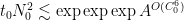
It seems natural to conjecture that similar triply logarithmic improvements can be made to several of the other blowup criteria listed above, but I have not attempted to pursue this question. It seems difficult to improve the triple logarithmic factor using only the techniques here; the Bourgain pigeonholing argument inevitably costs one exponential, the Carleman inequalities cost a second, and the stacking of scales at the end to contradict the upper bound costs the third.

 

Ultrafilters, nonstandard analysis, and epsilon management

This post is in some ways an antithesis of my previous postings on hard and soft analysis. In those posts, the emphasis was on taking a result in soft analysis and converting it into a hard analysis statement (making it more “quantitative” or “effective”); here we shall be focusing on the reverse procedure, in which one harnesses the power of infinitary mathematics – in particular, ultrafilters and nonstandard analysis – to facilitate the proof of finitary statements.

Arguments in hard analysis are notorious for their profusion of “epsilons and deltas”. In the more sophisticated arguments of this type, one can end up having an entire army of epsilons that one needs to manage, in particular choosing each epsilon carefully to be sufficiently small compared to other parameters (including other epsilons), while of course avoiding an impossibly circular situation in which a parameter is ultimately required to be small with respect to itself, which is absurd. This art of epsilon management, once mastered, is not terribly difficult – it basically requires one to mentally keep track of which quantities are “small”, “very small”, “very very small”, and so forth – but when these arguments get particularly lengthy, then epsilon management can get rather tedious, and also has the effect of making these arguments unpleasant to read. In particular, any given assertion in hard analysis usually comes with a number of unsightly quantifiers (For every there exists an N…) which can require some thought for a reader to parse. This is in contrast with soft analysis, in which most of the quantifiers (and the epsilons) can be cleanly concealed via the deployment of some very useful terminology; consider for instance how many quantifiers and epsilons are hidden within, say, the Heine-Borel theorem: “a subset of a Euclidean space is compact if and only if it is closed and bounded”.

For those who practice hard analysis for a living (such as myself), it is natural to wonder if one can somehow “clean up” or “automate” all the epsilon management which one is required to do, and attain levels of elegance and conceptual clarity comparable to those in soft analysis, hopefully without sacrificing too much of the “elementary” or “finitary” nature of hard analysis in the process.

A quantitative form of the Besicovitch projection theorem via multiscale analysis

I’ve just uploaded a new paper to the arXiv entitled “A quantitative form of the Besicovitch projection theorem via multiscale analysis“, submitted to the Journal of the London Mathematical Society. In the spirit of my earlier posts on soft and hard analysis, this paper establishes a quantitative version of a well-known theorem in soft analysis, in this case the Besicovitch projection theorem. This theorem asserts that if a subset E of the plane has finite length (in the Hausdorff sense) and is purely unrectifiable (thus its intersection with any Lipschitz graph has zero length), then almost every linear projection E to a line will have zero measure. (In contrast, if E is a rectifiable set of positive length, then it is easy to show that all but at most one linear projection of E will have positive measure, basically thanks to the Rademacher differentiation theorem.)

A concrete special case of this theorem relates to the product Cantor set K, consisting of all points (x,y) in the unit square whose base 4 expansion consists only of 0s and 3s. This is a compact one-dimensional set of finite length, which is purely unrectifiable, and so Besicovitch’s theorem tells us that almost every projection of K has measure zero. (One consequence of this, first observed by Kahane, is that one can construct Kakeya sets in the plane of zero measure by connecting line segments between one Cantor set and another.)

The Lebesgue differentiation theorem and the Szemeredi regularity lemma

This post is a sequel of sorts to my earlier post on hard and soft analysis, and the finite convergence principle. Here, I want to discuss a well-known theorem in infinitary soft analysis – the Lebesgue differentiation theorem – and whether there is any meaningful finitary version of this result. Along the way, it turns out that we will uncover a simple analogue of the Szemerédi regularity lemma, for subsets of the interval rather than for graphs. (Actually, regularity lemmas seem to appear in just about any context in which fine-scaled objects can be approximated by coarse-scaled ones.) The connection between regularity lemmas and results such as the Lebesgue differentiation theorem was recently highlighted by Elek and Szegedy, while the connection between the finite convergence principle and results such as the pointwise ergodic theorem (which is a close cousin of the Lebesgue differentiation theorem) was recently detailed by Avigad, Gerhardy, and Towsner.

The Lebesgue differentiation theorem has many formulations, but we will avoid the strongest versions and just stick to the following model case for simplicity:

Lebesgue differentiation theorem. If is Lebesgue measurable, then for almost every we have . Equivalently, the fundamental theorem of calculus is true for almost every x in [0,1].

Here we use the oriented definite integral, thus . Specialising to the case where is an indicator function, we obtain the Lebesgue density theorem as a corollary:

Lebesgue density theorem. Let be Lebesgue measurable. Then for almost every , we have as , where |A| denotes the Lebesgue measure of A.

In other words, almost all the points x of A are points of density of A, which roughly speaking means that as one passes to finer and finer scales, the immediate vicinity of x becomes increasingly saturated with A. (Points of density are like robust versions of interior points, thus the Lebesgue density theorem is an assertion that measurable sets are almost like open sets. This is Littlewood’s first principle.) One can also deduce the Lebesgue differentiation theorem back from the Lebesgue density theorem by approximating f by a finite linear combination of indicator functions; we leave this as an exercise.

Soft analysis, hard analysis, and the finite convergence principle

In the field of analysis, it is common to make a distinction between “hard”, “quantitative”, or “finitary” analysis on one hand, and “soft”, “qualitative”, or “infinitary” analysis on the other. “Hard analysis” is mostly concerned with finite quantities (e.g. the cardinality of finite sets, the measure of bounded sets, the value of convergent integrals, the norm of finite-dimensional vectors, etc.) and their quantitative properties (in particular, upper and lower bounds). “Soft analysis”, on the other hand, tends to deal with more infinitary objects (e.g. sequences, measurable sets and functions, -algebras, Banach spaces, etc.) and their qualitative properties (convergence, boundedness, integrability, completeness, compactness, etc.). To put it more symbolically, hard analysis is the mathematics of , , , and ^[1]; soft analysis is the mathematics of 0, , , and .

At first glance, the two types of analysis look very different; they deal with different types of objects, ask different types of questions, and seem to use different techniques in their proofs. They even use^[2] different axioms of mathematics; the axiom of infinity, the axiom of choice, and the Dedekind completeness axiom for the real numbers are often invoked in soft analysis, but rarely in hard analysis. (As a consequence, there are occasionally some finitary results that can be proven easily by soft analysis but are in fact impossible to prove via hard analysis methods; the Paris-Harrington theorem gives a famous example.) Because of all these differences, it is common for analysts to specialise in only one of the two types of analysis. For instance, as a general rule (and with notable exceptions), discrete mathematicians, computer scientists, real-variable harmonic analysts, and analytic number theorists tend to rely on “hard analysis” tools, whereas functional analysts, operator algebraists, abstract harmonic analysts, and ergodic theorists tend to rely on “soft analysis” tools. (PDE is an interesting intermediate case in which both types of analysis are popular and useful, though many practitioners of PDE still prefer to primarily use just one of the two types. Another interesting transition occurs on the interface between point-set topology, which largely uses soft analysis, and metric geometry, which largely uses hard analysis. Also, the ineffective bounds which crop up from time to time in analytic number theory are a sort of hybrid of hard and soft analysis. Finally, there are examples of evolution of a field from soft analysis to hard (e.g. Banach space geometry) or vice versa (e.g. recent developments in extremal combinatorics, particularly in relation to the regularity lemma).)