
You are currently browsing the monthly archive for August 2016.
This is a postscript to the previous blog post which was concerned with obtaining heuristic asymptotic predictions for the correlation

for the divisor function 
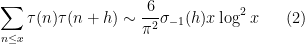
when 

for fixed 
is the order 


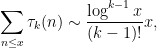
or more accurately
where 


for some polynomial 


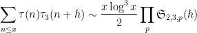
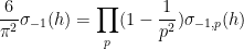
In principle, the calculations of the previous post should recover the predictions of Conrey and Gonek. In this post I would like to record this for the top order term:
Conjecture 1 If
and
are fixed, then
as
, where the product is over all primes
, and the local factors
are given by the formula
where
is the degree
polynomial
where
and one adopts the conventions that
and
for
.


For instance, if

and hence
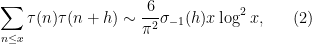
and the above conjecture recovers the Ingham formula (2). For 

and so we predict
where
Similarly, if 


and so we predict

where

and so forth.
As in the previous blog, the idea is to factorise
where the local factors 
(where 


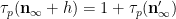
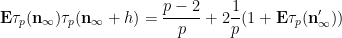
We then have the following exact local asymptotics:
Proposition 2 (Local correlations) Let
be a profinite integer chosen uniformly at random, let


(For profinite integers it is possible that 

Conjecture 1 can then be heuristically justified from the local calculations (2) by various pseudorandomness heuristics, as discussed in the previous post.
I’ll give a short proof of the above proposition below, basically using the recursive methods of the previous post. This short proof actually took be quite a while to find; I spent several hours and a fair bit of scratch paper working out the cases 

It was only after expending all this effort that I realised that it would be much more efficient to compute the correlations for all values of 
I am confident that Conjecture 1 is consistent with the explicit asymptotic in the Conrey-Gonek conjecture, but have not yet rigorously established that the leading order term in the latter is indeed identical to the expression provided above.
Let
where 


that is to say the random variable 


Now we turn to the pair correlations 

The error term in (2) has been refined by many subsequent authors, as has the uniformity of the estimates in the
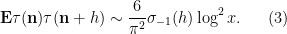
Using our probabilistic lens, the estimate (2) can be written as
From (1) (and the asymptotic negligibility of the shift by 


Ingham’s formula can be established in a number of ways. Firstly, one can expand out 


for various 


Each of the methods outlined above requires a fair amount of calculation, and it is not obvious while performing them that the factor 


using symmetry to order 


and we obtain the desired consistency after multiplying by
This still however does not explain the presence of the 
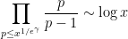
One heuristic way to proceed is through analysis of local factors. Observe from the fundamental theorem of arithmetic that we can factor
where the product is over all primes 


where
(or in terms of valuations, 


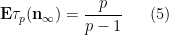
Proposition 1 (Local Ingham asymptotics) For fixed
and

From the Euler formula

we see that
and so one can “explain” the arithmetic factor 
Remark 2 The relation between the local means
and the global mean
can also be seen heuristically through the application
of Mertens’ theorem, where
is Pólya’s magic exponent, which serves as a useful heuristic limiting threshold in situations where the product of local factors is divergent.
Let us now prove this proposition. One could brute-force the computations by observing that for any fixed 

It is first convenient to get rid of error terms by observing that in the limit 


in the profinite setting (this setting will make it easier to set up the recursion).
We begin with (5). Observe that 


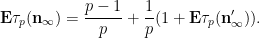
As 

We use a similar method to treat (6). First treat the case when 


and the claim (6) in this case follows from (5) and a brief computation (noting that 
Now suppose that 


which by (5) (and replacing

and (6) then follows by induction on the number of powers of
The estimate (2) of Ingham was refined by Estermann, who obtained the more accurate expansion


for certain complicated but explicit coefficients 

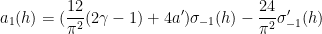
where 
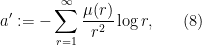
The formula for 


These lower order terms are traditionally computed either from a Dirichlet series approach (using Perron’s formula) or a circle method approach. It turns out that a refinement of the above heuristics can also predict these lower order terms, thus keeping the calculation purely in physical space as opposed to the “multiplicative frequency space” of the Dirichlet series approach, or the “additive frequency space” of the circle method, although the computations are arguably as messy as the latter computations for the purposes of working out the lower order terms. We illustrate this just for the 
Fifteen years ago, I wrote a paper entitled Global regularity of wave maps. II. Small energy in two dimensions, in which I established global regularity of wave maps from two spatial dimensions to the unit sphere, assuming that the initial data had small energy. Recently, Hao Jia (personal communication) discovered a small gap in the argument that requires a slightly non-trivial fix. The issue does not really affect the subsequent literature, because the main result has since been reproven and extended by methods that avoid the gap (see in particular this subsequent paper of Tataru), but I have decided to describe the gap and its fix on this blog.
I will assume familiarity with the notation of my paper. In Section 10, some complicated spaces ![{S[k] = S[k]({\bf R}^{1+n})}](https://s0.wp.com/latex.php?latex=%7BS%5Bk%5D+%3D+S%5Bk%5D%28%7B%5Cbf+R%7D%5E%7B1%2Bn%7D%29%7D&bg=ffffff&fg=000000&s=0&c=20201002)


} \ \ \ \ \ (1)](https://s0.wp.com/latex.php?latex=%5Cdisplaystyle++%5C%7C+%5Cphi+%5C%7C_%7BS%28c%29%28%7B%5Cbf+R%7D%5E%7B1%2Bn%7D%29%7D+%3A%3D+%5C%7C%5Cphi+%5C%7C_%7BL%5E%5Cinfty_t+L%5E%5Cinfty_x%28%7B%5Cbf+R%7D%5E%7B1%2Bn%7D%29%7D+%2B+%5Csup_k+c_k%5E%7B-1%7D+%5C%7C+%5Cphi_k+%5C%7C_%7BS%5Bk%5D%28%7B%5Cbf+R%7D%5E%7B1%2Bn%7D%29%7D+%5C+%5C+%5C+%5C+%5C+%281%29&bg=ffffff&fg=000000&s=0&c=20201002)
where 


![{[-T,T] \times {\bf R}^n}](https://s0.wp.com/latex.php?latex=%7B%5B-T%2CT%5D+%5Ctimes+%7B%5Cbf+R%7D%5En%7D&bg=ffffff&fg=000000&s=0&c=20201002)
![\displaystyle \| \phi \|_{S(c)([-T,T] \times {\bf R}^n)} := \inf \{ \| \tilde \phi \|_{S(c)({\bf R}^{1+n})}: \tilde \phi \downharpoonright_{[-T,T] \times {\bf R}^n} = \phi \}](https://s0.wp.com/latex.php?latex=%5Cdisplaystyle++%5C%7C+%5Cphi+%5C%7C_%7BS%28c%29%28%5B-T%2CT%5D+%5Ctimes+%7B%5Cbf+R%7D%5En%29%7D+%3A%3D+%5Cinf+%5C%7B+%5C%7C+%5Ctilde+%5Cphi+%5C%7C_%7BS%28c%29%28%7B%5Cbf+R%7D%5E%7B1%2Bn%7D%29%7D%3A+%5Ctilde+%5Cphi+%5Cdownharpoonright_%7B%5B-T%2CT%5D+%5Ctimes+%7B%5Cbf+R%7D%5En%7D+%3D+%5Cphi+%5C%7D&bg=ffffff&fg=000000&s=0&c=20201002)
where the infimum is taken over all extensions 

![\displaystyle \| \phi_k \|_{S_k([-T,T] \times {\bf R}^n)} := \inf \{ \| \tilde \phi_k \|_{S_k({\bf R}^{1+n})}: \tilde \phi_k \downharpoonright_{[-T,T] \times {\bf R}^n} = \phi_k \}.](https://s0.wp.com/latex.php?latex=%5Cdisplaystyle++%5C%7C+%5Cphi_k+%5C%7C_%7BS_k%28%5B-T%2CT%5D+%5Ctimes+%7B%5Cbf+R%7D%5En%29%7D+%3A%3D+%5Cinf+%5C%7B+%5C%7C+%5Ctilde+%5Cphi_k+%5C%7C_%7BS_k%28%7B%5Cbf+R%7D%5E%7B1%2Bn%7D%29%7D%3A+%5Ctilde+%5Cphi_k+%5Cdownharpoonright_%7B%5B-T%2CT%5D+%5Ctimes+%7B%5Cbf+R%7D%5En%7D+%3D+%5Cphi_k+%5C%7D.&bg=ffffff&fg=000000&s=0&c=20201002)
The gap in the paper is as follows: it was implicitly assumed that one could restrict (1) to the slab
![\displaystyle \| \phi \|_{S(c)([-T,T] \times {\bf R}^n)} = \|\phi \|_{L^\infty_t L^\infty_x([-T,T] \times {\bf R}^n)} + \sup_k c_k^{-1} \| \phi_k \|_{S[k]([-T,T] \times {\bf R}^n)}.](https://s0.wp.com/latex.php?latex=%5Cdisplaystyle++%5C%7C+%5Cphi+%5C%7C_%7BS%28c%29%28%5B-T%2CT%5D+%5Ctimes+%7B%5Cbf+R%7D%5En%29%7D+%3D+%5C%7C%5Cphi+%5C%7C_%7BL%5E%5Cinfty_t+L%5E%5Cinfty_x%28%5B-T%2CT%5D+%5Ctimes+%7B%5Cbf+R%7D%5En%29%7D+%2B+%5Csup_k+c_k%5E%7B-1%7D+%5C%7C+%5Cphi_k+%5C%7C_%7BS%5Bk%5D%28%5B-T%2CT%5D+%5Ctimes+%7B%5Cbf+R%7D%5En%29%7D.&bg=ffffff&fg=000000&s=0&c=20201002)
(This equality is implicitly used to establish the bound (36) in the paper.) Unfortunately, (1) only gives the lower bound, not the upper bound, and it is the upper bound which is needed here. The problem is that the extensions 

}}](https://s0.wp.com/latex.php?latex=%7B%5C%7C+%5Cphi_k+%5C%7C_%7BS%5Bk%5D%28%5B-T%2CT%5D+%5Ctimes+%7B%5Cbf+R%7D%5En%29%7D%7D&bg=ffffff&fg=000000&s=0&c=20201002)
![{\| \phi \|_{S(c)([-T,T] \times {\bf R}^n)}}](https://s0.wp.com/latex.php?latex=%7B%5C%7C+%5Cphi+%5C%7C_%7BS%28c%29%28%5B-T%2CT%5D+%5Ctimes+%7B%5Cbf+R%7D%5En%29%7D%7D&bg=ffffff&fg=000000&s=0&c=20201002)
To remedy the problem, one has to prove an upper bound of the form
![\displaystyle \| \phi \|_{S(c)([-T,T] \times {\bf R}^n)} \lesssim \|\phi \|_{L^\infty_t L^\infty_x([-T,T] \times {\bf R}^n)} + \sup_k c_k^{-1} \| \phi_k \|_{S[k]([-T,T] \times {\bf R}^n)}](https://s0.wp.com/latex.php?latex=%5Cdisplaystyle++%5C%7C+%5Cphi+%5C%7C_%7BS%28c%29%28%5B-T%2CT%5D+%5Ctimes+%7B%5Cbf+R%7D%5En%29%7D+%5Clesssim+%5C%7C%5Cphi+%5C%7C_%7BL%5E%5Cinfty_t+L%5E%5Cinfty_x%28%5B-T%2CT%5D+%5Ctimes+%7B%5Cbf+R%7D%5En%29%7D+%2B+%5Csup_k+c_k%5E%7B-1%7D+%5C%7C+%5Cphi_k+%5C%7C_%7BS%5Bk%5D%28%5B-T%2CT%5D+%5Ctimes+%7B%5Cbf+R%7D%5En%29%7D&bg=ffffff&fg=000000&s=0&c=20201002)
for all Schwartz
![\displaystyle \|\phi \|_{L^\infty_t L^\infty_x([-T,T] \times {\bf R}^n)} \leq 1 \ \ \ \ \ (2)](https://s0.wp.com/latex.php?latex=%5Cdisplaystyle++%5C%7C%5Cphi+%5C%7C_%7BL%5E%5Cinfty_t+L%5E%5Cinfty_x%28%5B-T%2CT%5D+%5Ctimes+%7B%5Cbf+R%7D%5En%29%7D+%5Cleq+1+%5C+%5C+%5C+%5C+%5C+%282%29&bg=ffffff&fg=000000&s=0&c=20201002)
} \leq c_k \ \ \ \ \ (3)](https://s0.wp.com/latex.php?latex=%5Cdisplaystyle++%5C%7CP_k+%5Cphi+%5C%7C_%7BS%5Bk%5D%28%5B-T%2CT%5D+%5Ctimes+%7B%5Cbf+R%7D%5En%29%7D+%5Cleq+c_k+%5C+%5C+%5C+%5C+%5C+%283%29&bg=ffffff&fg=000000&s=0&c=20201002)
for each

} \lesssim c_k \ \ \ \ \ (5)](https://s0.wp.com/latex.php?latex=%5Cdisplaystyle++%5C%7CP_k+%5Ctilde+%5Cphi+%5C%7C_%7BS%5Bk%5D%28%7B%5Cbf+R%7D%5E%7B1%2Bn%7D%29%7D+%5Clesssim+c_k+%5C+%5C+%5C+%5C+%5C+%285%29&bg=ffffff&fg=000000&s=0&c=20201002)
for each 
} \lesssim c_k; \ \ \ \ \ (6)](https://s0.wp.com/latex.php?latex=%5Cdisplaystyle++%5C%7C%5Ctilde+%5Cphi_k+%5C%7C_%7BS%5Bk%5D%28%7B%5Cbf+R%7D%5E%7B1%2Bn%7D%29%7D+%5Clesssim+c_k%3B+%5C+%5C+%5C+%5C+%5C+%286%29&bg=ffffff&fg=000000&s=0&c=20201002)
the extension 
![{S[k]}](https://s0.wp.com/latex.php?latex=%7BS%5Bk%5D%7D&bg=ffffff&fg=000000&s=0&c=20201002)


This can be fixed as follows. For each 
![{[-T-2^{-k}, T+2^{-k}]}](https://s0.wp.com/latex.php?latex=%7B%5B-T-2%5E%7B-k%7D%2C+T%2B2%5E%7B-k%7D%5D%7D&bg=ffffff&fg=000000&s=0&c=20201002)
![{[-T-2^{-k-1},T+2^{-k+1}]}](https://s0.wp.com/latex.php?latex=%7B%5B-T-2%5E%7B-k-1%7D%2CT%2B2%5E%7B-k%2B1%7D%5D%7D&bg=ffffff&fg=000000&s=0&c=20201002)


} \lesssim \| \tilde \phi_k \|_{S[k]({\bf R}^{1+n})}. \ \ \ \ \ (7)](https://s0.wp.com/latex.php?latex=%5Cdisplaystyle++%5C%7C+%5Ceta_k+%5Ctilde+%5Cphi_k+%5C%7C_%7BS%5Bk%5D%28%7B%5Cbf+R%7D%5E%7B1%2Bn%7D%29%7D+%5Clesssim+%5C%7C+%5Ctilde+%5Cphi_k+%5C%7C_%7BS%5Bk%5D%28%7B%5Cbf+R%7D%5E%7B1%2Bn%7D%29%7D.+%5C+%5C+%5C+%5C+%5C+%287%29&bg=ffffff&fg=000000&s=0&c=20201002)
Assuming this estimate, then if we set 

for all 
For ![{t \in [-T,T]}](https://s0.wp.com/latex.php?latex=%7Bt+%5Cin+%5B-T%2CT%5D%7D&bg=ffffff&fg=000000&s=0&c=20201002)
![{t \in [T+2^{k_0-1}, T+2^{k_0}]}](https://s0.wp.com/latex.php?latex=%7Bt+%5Cin+%5BT%2B2%5E%7Bk_0-1%7D%2C+T%2B2%5E%7Bk_0%7D%5D%7D&bg=ffffff&fg=000000&s=0&c=20201002)

![{t \in [-T-2^{k_0}, -T-2^{k_0-1}]}](https://s0.wp.com/latex.php?latex=%7Bt+%5Cin+%5B-T-2%5E%7Bk_0%7D%2C+-T-2%5E%7Bk_0-1%7D%5D%7D&bg=ffffff&fg=000000&s=0&c=20201002)

where

The contribution of the 


By hypothesis, 
} \lesssim 2^k;](https://s0.wp.com/latex.php?latex=%5Cdisplaystyle++%5C%7C+%5Cpartial_t+%5Ctilde+%5Cphi_k+%5C%7C_%7BL%5E%5Cinfty_t+L%5E%5Cinfty_x%28%7B%5Cbf+R%7D%5E%7B1%2Bn%7D%29%7D+%5Clesssim+2%5Ek+%5C%7C+%5Ctilde+%5Cphi_k+%5C%7C_%7BS%5Bk%5D%28%7B%5Cbf+R%7D%5E%7B1%2Bn%7D%29%7D+%5Clesssim+2%5Ek%3B&bg=ffffff&fg=000000&s=0&c=20201002)
and then we are done by summing the geometric series in
It remains to prove the truncation estimate (7). This estimate is similar in spirit to the algebra estimates already in my paper, but unfortunately does not seem to follow immediately from these estimates as written, and so one has to repeat the somewhat lengthy decompositions and case checkings used to prove these estimates. We do this below the fold.
[This blog post was written jointly by Terry Tao and Will Sawin.]
In the previous blog post, one of us (Terry) implicitly introduced a notion of rank for tensors which is a little different from the usual notion of tensor rank, and which (following BCCGNSU) we will call “slice rank”. This notion of rank could then be used to encode the Croot-Lev-Pach-Ellenberg-Gijswijt argument that uses the polynomial method to control capsets.
Afterwards, several papers have applied the slice rank method to further problems – to control tri-colored sum-free sets in abelian groups (BCCGNSU, KSS) and from there to the triangle removal lemma in vector spaces over finite fields (FL), to control sunflowers (NS), and to bound progression-free sets in
In this post we investigate the notion of slice rank more systematically. In particular, we show how to give lower bounds for the slice rank. In many cases, we can show that the upper bounds on slice rank given in the aforementioned papers are sharp to within a subexponential factor. This still leaves open the possibility of getting a better bound for the original combinatorial problem using the slice rank of some other tensor, but for very long arithmetic progressions (at least eight terms), we show that the slice rank method cannot improve over the trivial bound using any tensor.
It will be convenient to work in a “basis independent” formalism, namely working in the category of abstract finite-dimensional vector spaces over a fixed field 


defined in the obvious fashion. Elements of 


For 


From basic linear algebra we have the following equivalences:
Lemma 1 Let
, and let
- (i) One has
.
- (ii) One has a representation of the form
where
are finite sets of total cardinality
at most
,
and
.
- (iii) One has
where for each
,
is a subspace of
of total dimension
at most
as a subspace of
- (iv) (Dual formulation) There exist subspaces
of the dual space
for
, such that
, in the sense that one has the vanishing
for all
, where
is the obvious pairing.


Proof: The equivalence of (i) and (ii) is clear from definition. To get from (ii) to (iii) one simply takes 


One corollary of the formulation (iv), is that the set of tensors of slice rank at most 
Corollary 2 Let
be finite-dimensional vector spaces over an algebraically closed field
Proof: In view of Lemma 1(i and iv), this set is the union over tuples of integers 


One can check directly that the set of tuples 

We also have good behaviour with respect to linear transformations:
Lemma 3 Let
be finite-dimensional vector spaces over a field
be a linear transformation, with
the tensor product of these maps. Then
Furthermore, if the
are all injective, then one has equality in (2).

Thus, for instance, the rank of a tensor 
Proof: The bound (2) is clear from the formulation (ii) of rank in Lemma 1. For equality, apply (2) to the injective 
Computing the rank of a tensor is difficult in general; however, the problem becomes a combinatorial one if one has a suitably sparse representation of that tensor in some basis, where we will measure sparsity by the property of being an antichain.
Proposition 4 Let
be a linearly independent set in
. Let
be a subset of
.
where for each
,
is a coefficient in
where the minimum ranges over all coverings of
, and
for
Now suppose that the coefficients
, and
is the set of maximal elements of
,
such that
for all
In particular, if


Proof: By Lemma 3 (or by enlarging the bases 
with the usual ordering, and by Lemma 3 we may take each 

Let

for any covering of 

can (after collecting terms) be written as

for some 
Now assume that the

holds for some 

Let 


such that for all 


We now claim that 


As
for any tuple 


plus a linear combination of other tensor products 


For each 


As an instance of this proposition, we recover the computation of diagonal rank from the previous blog post:
Example 5 Let
. Let
be a linearly independent set in
be non-zero coefficients in
has rank
, with
the standard ordering, and another of the
are all bijective, and so it is clear that the minimum in (4) is simply

The combinatorial minimisation problem in the above proposition can be solved asymptotically when working with tensor powers, using the notion of the Shannon entropy 

Proposition 6 Let
Let
be a tensor of the form (3) for some coefficients
be the tensor power of
. Then
and
range over the random variables taking values in
Now suppose that the coefficients
where
as
. In particular, if the maximizer in (10) is supported on the maximal elements of


Proof:

as 


We first prove the lower bound. By compactness (and the continuity properties of entropy), we can find a random variable

Let 


By the asymptotic equipartition property, the cardinality of 

if

 , one has
Now let 

which by (13) implies that

noting that the 

Now we prove the upper bound. We can cover 


for all 
It is of interest to compute the quantity 
Proposition 7 Let
be non-empty. Let
denote the essential range of
such that
is non-zero. Then the following are equivalent:
- (i)
- (ii) There exist weights
and a finite quantity
, such that
whenever
, and such that
for all
. (In particular,
must vanish if there exists a
with
.)
Furthermore, when (i) and (ii) holds, one has

Proof: We first show that (i) implies (ii). The function 
![{[0,1]}](https://s0.wp.com/latex.php?latex=%7B%5B0%2C1%5D%7D&bg=ffffff&fg=000000&s=0&c=20201002)


where 


By construction, the quantity

is maximised when 


for sufficiently small 

for small
and similarly for 


almost surely; taking expectations we conclude that
The inner sum is 
Now we show conversely that (ii) implies (i). As noted previously, the function 

for any 


By construction, one has
and

so to prove that 

or equivalently that the quantity

is maximised when

it suffices to show this claim for the quantity
One can view this quantity as

By (ii), this quantity is bounded by
The second half of the proof of Proposition 7 only uses the marginal distributions 
Remark 8 Suppose one is in the situation of (i) and (ii) above; assume the nondegeneracy condition that
to each element
then every tuple
, and hence by (17), each such tuple has a
for some
. On the other hand, we can compute from (19) and the fact that
for
that
. Thus, by asymptotic equipartition, and assuming
; one can in fact use (19) and (18) to show that this is in fact an equality. This gives a direct way to cover
with
, which is in the spirit of the Croot-Lev-Pach-Ellenberg-Gijswijt arguments from the previous post.

We can now show that the rank computation for the capset problem is sharp:
Proposition 9 Let
denote the space of functions from
to
. Then the function
from
to
, has rank
as
is given by the formula


Proof: In 


Thus, if we let 


of 


then 


To compute the quantity at (10), we use the criterion in Proposition 7. We take 


we can verify the condition (16) with equality for all 

This statement already follows from the result of Kleinberg-Sawin-Speyer, which gives a “tri-colored sum-free set” in 

We can also show that the slice rank upper bound in a result of Naslund-Sawin is similarly sharp:
Proposition 10 Let
to
. Then the function
from
, viewed as an element of

Proof: Let 


Set 


Let 


Setting 


We used a slightly different method in each of the last two results. In the first one, we use the most natural bases for all three vector spaces, and distinguish 


Proposition 11 Let
be a natural number and let
be a finite abelian group. Let
denote the space of functions from
Let
be any
that is nonzero only when the
form a
Then the slice rank of
.
Proof: We apply Proposition 4, using the standard bases of 


So it is sufficient to find 

So it is sufficient to find 

Then let 

![{c \in [0, (n-1)/2]}](https://s0.wp.com/latex.php?latex=%7Bc+%5Cin+%5B0%2C+%28n-1%29%2F2%5D%7D&bg=ffffff&fg=000000&s=0&c=20201002)

![{c \in [0,(n-1)/2]}](https://s0.wp.com/latex.php?latex=%7Bc+%5Cin+%5B0%2C%28n-1%29%2F2%5D%7D&bg=ffffff&fg=000000&s=0&c=20201002)
Take a representative of the residue class 
![{[-n/2,n/2]}](https://s0.wp.com/latex.php?latex=%7B%5B-n%2F2%2Cn%2F2%5D%7D&bg=ffffff&fg=000000&s=0&c=20201002)


![{[0,c]}](https://s0.wp.com/latex.php?latex=%7B%5B0%2Cc%5D%7D&bg=ffffff&fg=000000&s=0&c=20201002)


![{[mn,mn+c]}](https://s0.wp.com/latex.php?latex=%7B%5Bmn%2Cmn%2Bc%5D%7D&bg=ffffff&fg=000000&s=0&c=20201002)


In fact, given a

Recent Comments