
You are currently browsing the monthly archive for October 2017.
In 2010, the UCLA mathematics department launched a scholarship opportunity for entering freshman students with exceptional background and promise in mathematics. We are able to offer one scholarship each year. The UCLA Math Undergraduate Merit Scholarship provides for full tuition, and a room and board allowance for 4 years, contingent on continued high academic performance. In addition, scholarship recipients follow an individualized accelerated program of study, as determined after consultation with UCLA faculty. The program of study leads to a Masters degree in Mathematics in four years.
More information and an application form for the scholarship can be found on the web at:
http://www.math.ucla.edu/ugrad/mums
To be considered for Fall 2018, candidates must apply for the scholarship and also for admission to UCLA on or before November 30, 2017.
Let 


for all 


For 

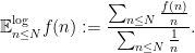
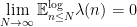
In recent years, it has been realised that one can make more progress on this conjecture if one works instead with the logarithmically averaged version

of the conjecture, where we use the logarithmic averaging notation
Using the summation by parts (or telescoping series) identity
it is not difficult to show that the Chowla conjecture (1) for a given 
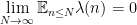
is equivalent to the prime number theorem; but the logarithmically averaged analogue
is significantly easier to show (a proof with the Liouville function 


In view of this emerging consensus that the logarithmically averaged Chowla conjecture was easier than the ordinary Chowla conjecture, it was thus somewhat of a surprise for me to read a recent paper of Gomilko, Kwietniak, and Lemanczyk who (among other things) established the following statement:
Theorem 1 Assume that the logarithmically averaged Chowla conjecture (2) is true for all
going to infinity such that the Chowla conjecture (1) is true for all
for all

This implication does not use any special properties of the Liouville function (other than that they are bounded), and in fact proceeds by ergodic theoretic methods, focusing in particular on the ergodic decomposition of invariant measures of a shift into ergodic measures. Ergodic methods have proven remarkably fruitful in understanding these sorts of number theoretic and combinatorial problems, as could already be seen by the ergodic theoretic proof of Szemerédi’s theorem by Furstenberg, and more recently by the work of Frantzikinakis and Host on Sarnak’s conjecture. (My first paper with Teravainen also uses ergodic theory tools.) Indeed, many other results in the subject were first discovered using ergodic theory methods.
On the other hand, many results in this subject that were first proven ergodic theoretically have since been reproven by more combinatorial means; my second paper with Teravainen is an instance of this. As it turns out, one can also prove Theorem 1 by a standard combinatorial (or probabilistic) technique known as the second moment method. In fact, one can prove slightly more:
Theorem 2 Let
. Then there exists a set
of natural numbers of logarithmic density
(that is,
) such that
for any distinct

It is not difficult to deduce Theorem 1 from Theorem 2 using a diagonalisation argument. Unfortunately, the known cases of the logarithmically averaged Chowla conjecture (
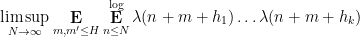
We now sketch the proof of Theorem 2. For any distinct 

We can expand this as

If all the 


By Markov’s inequality (and (3)), we conclude that for any fixed 


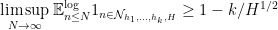
such that

By deleting at most finitely many elements, we may assume that 
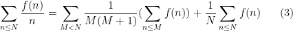
For any 


for some 

interchanging the sums and using

We conclude on taking

as required.
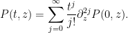
Let 


for some complex zeroes 
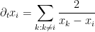
Now suppose we evolve 

On the space of polynomials of degree at most 
For instance, if one starts with a quadratic 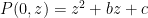

As the polynomial 

For instance, in the quadratic case, the quadratic formula tells us that the zeroes are

and
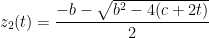
after arbitrarily choosing a branch of the square root. If 


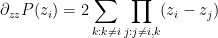
In the general case, we can obtain the equations of motion by implicitly differentiating the defining equation

in time using (2) to obtain

To simplify notation we drop the explicit dependence on time, thus

From (1) and the product rule, we see that

and
(where all indices are understood to range over 

at least when one avoids those times in which there is a repeated zero. In the case when the zeroes 


One interesting consequence of these equations is that if the zeroes are real at some time, then they will stay real as long as the zeroes do not collide. Let us now restrict attention to the case of real simple zeroes, in which case we will rename the zeroes as 

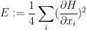
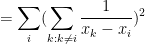
can now be thought of as reverse gradient flow for the “entropy”

(which is also essentially the logarithm of the discriminant of the polynomial) since we have

In particular, we have the monotonicity formula

where 
where in the last line we use the antisymmetrisation identity

Among other things, this shows that as one goes backwards in time, the entropy decreases, and so no collisions can occur to the past, only in the future, which is of course consistent with the attractive nature of the dynamics. As 
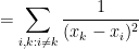
Exercise 1 Show that

Symmetric polynomials of the zeroes are polynomial functions of the coefficients and should thus evolve in a polynomial fashion. One can compute this explicitly in simple cases. For instance, the center of mass is an invariant:

The variance decreases linearly:
Exercise 2 Establish the virial identity
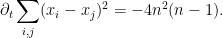
As the variance (which is proportional to 

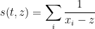
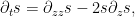
Exercise 3 Show that the Stieltjes transform
solves the viscous Burgers equation
either by using the original heat equation (2) and the identity
, or else by using the equations of motion (3). This relation between the Burgers equation and the heat equation is known as the Cole-Hopf transformation.
The paper of Csordas, Smith, and Varga mentioned previously gives some other bounds on the lifespan of the dynamics; roughly speaking, they show that if there is one pair of zeroes that are much closer to each other than to the other zeroes then they must collide in a short amount of time (unless there is a collision occuring even earlier at some other location). Their argument extends also to situations where there are an infinite number of zeroes, which they apply to get new results on Newman’s conjecture in analytic number theory. I would be curious to know of further places in the literature where this dynamics has been studied.
Joni Teräväinen and I have just uploaded to the arXiv our paper “Odd order cases of the logarithmically averaged Chowla conjecture“, submitted to J. Numb. Thy. Bordeaux. This paper gives an alternate route to one of the main results of our previous paper, and more specifically reproves the asymptotic
for all odd 


Recent Comments