A cheap version of Halasz’s inequality

A basic estimate in multiplicative number theory (particularly if one is using the Granville-Soundararajan “pretentious” approach to this subject) is the following inequality of Halasz (formulated here in a quantitative form introduced by Montgomery and Tenenbaum).

Theorem 1 (Halasz inequality) Let be a multiplicative function bounded in magnitude by , and suppose that , , and are such that

for all real numbers with . Then

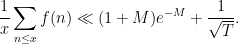
As a qualitative corollary, we conclude (by standard compactness arguments) that if

for all real , then

as . In the more recent work of this paper of Granville and Soundararajan, the sharper bound

is obtained (with a more precise description of the term).

The usual proofs of Halasz’s theorem are somewhat lengthy (though there has been a recent simplification, in forthcoming work of Granville, Harper, and Soundarajan). Below the fold I would like to give a relatively short proof of the following “cheap” version of the inequality, which has slightly weaker quantitative bounds, but still suffices to give qualitative conclusions such as (2).

Theorem 2 (Cheap Halasz inequality) Let be a multiplicative function bounded in magnitude by . Let and , and suppose that is sufficiently large depending on . If (1) holds for all , then

The non-optimal exponent can probably be improved a bit by being more careful with the exponents, but I did not try to optimise it here. A similar bound appears in the first paper of Halasz on this topic.

The idea of the argument is to split as a Dirichlet convolution where is the portion of coming from “small”, “medium”, and “large” primes respectively (with the dividing line between the three types of primes being given by various powers of ). Using a Perron-type formula, one can express this convolution in terms of the product of the Dirichlet series of respectively at various complex numbers with . One can use based estimates to control the Dirichlet series of , while using the hypothesis (1) one can get estimates on the Dirichlet series of . (This is similar to the Fourier-analytic approach to ternary additive problems, such as Vinogradov’s theorem on representing large odd numbers as the sum of three primes.) This idea was inspired by a similar device used in the work of Granville, Harper, and Soundarajan. A variant of this argument also appears in unpublished work of Adam Harper.

I thank Andrew Granville for helpful comments which led to significant simplifications of the argument.

275A, Notes 5: Variants of the central limit theorem

In the previous set of notes we established the central limit theorem, which we formulate here as follows:

Theorem 1 (Central limit theorem) Let be iid copies of a real random variable of mean and variance , and write . Then, for any fixed , we have

as .

This is however not the end of the matter; there are many variants, refinements, and generalisations of the central limit theorem, and the purpose of this set of notes is to present a small sample of these variants.

First of all, the above theorem does not quantify the rate of convergence in (1). We have already addressed this issue to some extent with the Berry-Esséen theorem, which roughly speaking gives a convergence rate of uniformly in if we assume that has finite third moment. However there are still some quantitative versions of (1) which are not addressed by the Berry-Esséen theorem. For instance one may be interested in bounding the large deviation probabilities

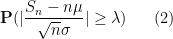
in the setting where grows with . Chebyshev’s inequality gives an upper bound of for this quantity, but one can often do much better than this in practice. For instance, the central limit theorem (1) suggests that this probability should be bounded by something like ; however, this theorem only kicks in when is very large compared with . For instance, if one uses the Berry-Esséen theorem, one would need as large as or so to reach the desired bound of , even under the assumption of finite third moment. Basically, the issue is that convergence-in-distribution results, such as the central limit theorem, only really control the typical behaviour of statistics in ; they are much less effective at controlling the very rare outlier events in which the statistic strays far from its typical behaviour. Fortunately, there are large deviation inequalities (or concentration of measure inequalities) that do provide exponential type bounds for quantities such as (2), which are valid for both small and large values of . A basic example of this is the Chernoff bound that made an appearance in Exercise 47 of Notes 4; here we give some further basic inequalities of this type, including versions of the Bennett and Hoeffding inequalities.

In the other direction, we can also look at the fine scale behaviour of the sums by trying to control probabilities such as

where is now bounded (but can grow with ). The central limit theorem predicts that this quantity should be roughly , but even if one is able to invoke the Berry-Esséen theorem, one cannot quite see this main term because it is dominated by the error term in Berry-Esséen. There is good reason for this: if for instance takes integer values, then also takes integer values, and can vanish when is less than and is slightly larger than an integer. However, this turns out to essentially be the only obstruction; if does not lie in a lattice such as , then we can establish a local limit theorem controlling (3), and when does take values in a lattice like , there is a discrete local limit theorem that controls probabilities such as . Both of these limit theorems will be proven by the Fourier-analytic method used in the previous set of notes.

We also discuss other limit theorems in which the limiting distribution is something other than the normal distribution. Perhaps the most common example of these theorems is the Poisson limit theorems, in which one sums a large number of indicator variables (or approximate indicator variables), each of which is rarely non-zero, but which collectively add up to a random variable of medium-sized mean. In this case, it turns out that the limiting distribution should be a Poisson random variable; this again is an easy application of the Fourier method. Finally, we briefly discuss limit theorems for other stable laws than the normal distribution, which are suitable for summing random variables of infinite variance, such as the Cauchy distribution.

Finally, we mention a very important class of generalisations to the CLT (and to the variants of the CLT discussed in this post), in which the hypothesis of joint independence between the variables is relaxed, for instance one could assume only that the form a martingale. Many (though not all) of the proofs of the CLT extend to these more general settings, and this turns out to be important for many applications in which one does not expect joint independence. However, we will not discuss these generalisations in this course, as they are better suited for subsequent courses in this series when the theory of martingales, conditional expectation, and related tools are developed.

Chains of large gaps between primes

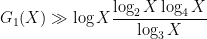
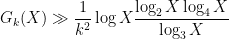
Kevin Ford, James Maynard, and I have uploaded to the arXiv our preprint “Chains of large gaps between primes“. This paper was announced in our previous paper with Konyagin and Green, which was concerned with the largest gap

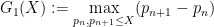
between consecutive primes up to , in which we improved the Rankin bound of

to

for large (where we use the abbreviations , , and ). Here, we obtain an analogous result for the quantity

which measures how far apart the gaps between chains of consecutive primes can be. Our main result is

whenever is sufficiently large depending on , with the implied constant here absolute (and effective). The factor of is inherent to the method, and related to the basic probabilistic fact that if one selects numbers at random from the unit interval , then one expects the minimum gap between adjacent numbers to be about (i.e. smaller than the mean spacing of by an additional factor of ).

Our arguments combine those from the previous paper with the matrix method of Maier, who (in our notation) showed that

for an infinite sequence of going to infinity. (Maier needed to restrict to an infinite sequence to avoid Siegel zeroes, but we are able to resolve this issue by the now standard technique of simply eliminating a prime factor of an exceptional conductor from the sieve-theoretic portion of the argument. As a byproduct, this also makes all of the estimates in our paper effective.)

As its name suggests, the Maier matrix method is usually presented by imagining a matrix of numbers, and using information about the distribution of primes in the columns of this matrix to deduce information about the primes in at least one of the rows of the matrix. We found it convenient to interpret this method in an equivalent probabilistic form as follows. Suppose one wants to find an interval which contained a block of at least primes, each separated from each other by at least (ultimately, will be something like and something like ). One can do this by the probabilistic method: pick to be a random large natural number (with the precise distribution to be chosen later), and try to lower bound the probability that the interval contains at least primes, no two of which are within of each other.

By carefully choosing the residue class of with respect to small primes, one can eliminate several of the from consideration of being prime immediately. For instance, if is chosen to be large and even, then the with even have no chance of being prime and can thus be eliminated; similarly if is large and odd, then cannot be prime for any odd . Using the methods of our previous paper, we can find a residue class (where is a product of a large number of primes) such that, if one chooses to be a large random element of (that is, for some large random integer ), then the set of shifts for which still has a chance of being prime has size comparable to something like ; furthermore this set is fairly well distributed in in the sense that it does not concentrate too strongly in any short subinterval of . The main new difficulty, not present in the previous paper, is to get lower bounds on the size of in addition to upper bounds, but this turns out to be achievable by a suitable modification of the arguments.

Using a version of the prime number theorem in arithmetic progressions due to Gallagher, one can show that for each remaining shift , is going to be prime with probability comparable to , so one expects about primes in the set . An upper bound sieve (e.g. the Selberg sieve) also shows that for any distinct , the probability that and are both prime is . Using this and some routine second moment calculations, one can then show that with large probability, the set will indeed contain about primes, no two of which are closer than to each other; with no other numbers in this interval being prime, this gives a lower bound on .

Klaus Roth

Klaus Roth, who made fundamental contributions to analytic number theory, died this Tuesday, aged 90.

I never met or communicated with Roth personally, but was certainly influenced by his work; he wrote relatively few papers, but they tended to have outsized impact. For instance, he was one of the key people (together with Bombieri) to work on simplifying and generalising the large sieve, taking it from the technically formidable original formulation of Linnik and Rényi to the clean and general almost orthogonality principle that we have today (discussed for instance in these lecture notes of mine). The paper of Roth that had the most impact on my own personal work was his three-page paper proving what is now known as Roth’s theorem on arithmetic progressions:

Theorem 1 (Roth’s theorem on arithmetic progressions) Let be a set of natural numbers of positive upper density (thus ). Then contains infinitely many arithmetic progressions of length three (with non-zero of course).

At the heart of Roth’s elegant argument was the following (surprising at the time) dichotomy: if had some moderately large density within some arithmetic progression , either one could use Fourier-analytic methods to detect the presence of an arithmetic progression of length three inside , or else one could locate a long subprogression of on which had increased density. Iterating this dichotomy by an argument now known as the density increment argument, one eventually obtains Roth’s theorem, no matter which side of the dichotomy actually holds. This argument (and the many descendants of it), based on various “dichotomies between structure and randomness”, became essential in many other results of this type, most famously perhaps in Szemerédi’s proof of his celebrated theorem on arithmetic progressions that generalised Roth’s theorem to progressions of arbitrary length. More recently, my recent work on the Chowla and Elliott conjectures that was a crucial component of the solution of the Erdös discrepancy problem, relies on an entropy decrement argument which was directly inspired by the density increment argument of Roth.

The Erdös discrepancy problem also is connected with another well known theorem of Roth:

Theorem 2 (Roth’s discrepancy theorem for arithmetic progressions) Let be a sequence in . Then there exists an arithmetic progression in with positive such that

for an absolute constant .

In fact, Roth proved a stronger estimate regarding mean square discrepancy, which I am not writing down here; as with the Roth theorem in arithmetic progressions, his proof was short and Fourier-analytic in nature (although non-Fourier-analytic proofs have since been found, for instance the semidefinite programming proof of Lovasz). The exponent is known to be sharp (a result of Matousek and Spencer).

As a particular corollary of the above theorem, for an infinite sequence of signs, the sums are unbounded in . The Erdös discrepancy problem asks whether the same statement holds when is restricted to be zero. (Roth also established discrepancy theorems for other sets, such as rectangles, which will not be discussed here.)

Finally, one has to mention Roth’s most famous result, cited for instance in his Fields medal citation:

Theorem 3 (Roth’s theorem on Diophantine approximation) Let be an irrational algebraic number. Then for any there is a quantity such that

From the Dirichlet approximation theorem (or from the theory of continued fractions) we know that the exponent in the denominator cannot be reduced to or below. A classical and easy theorem of Liouville gives the claim with the exponent replaced by the degree of the algebraic number ; work of Thue and Siegel reduced this exponent, but Roth was the one who obtained the near-optimal result. An important point is that the constant is ineffective – it is a major open problem in Diophantine approximation to produce any bound significantly stronger than Liouville’s theorem with effective constants. This is because the proof of Roth’s theorem does not exclude any single rational from being close to , but instead very ingeniously shows that one cannot have two different rationals , that are unusually close to , even when the denominators are very different in size. (I refer to this sort of argument as a “dueling conspiracies” argument; they are strangely prevalent throughout analytic number theory.)

Analytic number theory program at MSRI: Jan-May 2017 (second announcement)

Chantal David, Andrew Granville, Emmanuel Kowalski, Phillipe Michel, Kannan Soundararajan, and I are running a program at MSRI in the Spring of 2017 (more precisely, from Jan 17, 2017 to May 26, 2017) in the area of analytic number theory, with the intention to bringing together many of the leading experts in all aspects of the subject and to present recent work on the many active areas of the subject (e.g. the distribution of the prime numbers, refinements of the circle method, a deeper understanding of the asymptotics of bounded multiplicative functions (and applications to Erdos discrepancy type problems!) and of the “pretentious” approach to analytic number theory, more “analysis-friendly” formulations of the theorems of Deligne and others involving trace functions over fields, and new subconvexity theorems for automorphic forms, to name a few).  Like any other semester MSRI program, there will be a number of workshops, seminars, and similar activities taking place while the members are in residence.  I’m personally looking forward to the program, which should be occurring in the midst of a particularly productive time for the subject.  Needless to say, I (and the rest of the organising committee) plan to be present for most of the program.

Applications for Postdoctoral Fellowships and Research Memberships for this program (and for other MSRI programs in this time period, namely the companion program in Harmonic Analysis and the Fall program in Geometric Group Theory, as well as the complementary program in all other areas of mathematics) remain open until Dec 1.  Applications are open to everyone, but require supporting documentation, such as a CV, statement of purpose, and letters of recommendation from other mathematicians; see the application page for more details.

275A, Notes 4: The central limit theorem

Let be iid copies of an absolutely integrable real scalar random variable , and form the partial sums . As we saw in the last set of notes, the law of large numbers ensures that the empirical averages converge (both in probability and almost surely) to a deterministic limit, namely the mean of the reference variable . Furthermore, under some additional moment hypotheses on the underlying variable , we can obtain square root cancellation for the fluctuation of the empirical average from the mean. To simplify the calculations, let us first restrict to the case of mean zero and variance one, thus

and

Then, as computed in previous notes, the normalised fluctuation also has mean zero and variance one:

This and Chebyshev’s inequality already indicates that the “typical” size of is , thus for instance goes to zero in probability for any that goes to infinity as . If we also have a finite fourth moment , then the calculations of the previous notes also give a fourth moment estimate

From this and the Paley-Zygmund inequality (Exercise 44 of Notes 1) we also get some lower bound for of the form

for some absolute constant and for sufficiently large; this indicates in particular that does not converge in any reasonable sense to something finite for any that goes to infinity.
The question remains as to what happens to the ratio itself, without multiplying or dividing by any factor . A first guess would be that these ratios converge in probability or almost surely, but this is unfortunately not the case:

Proposition 1 Let be iid copies of an absolutely integrable real scalar random variable with mean zero, variance one, and finite fourth moment, and write . Then the random variables do not converge in probability or almost surely to any limit, and neither does any subsequence of these random variables.

Proof: Suppose for contradiction that some sequence converged in probability or almost surely to a limit . By passing to a further subsequence we may assume that the convergence is in the almost sure sense. Since all of the have mean zero, variance one, and bounded fourth moment, Theorem 25 of Notes 1 implies that the limit also has mean zero and variance one. On the other hand, is a tail random variable and is thus almost surely constant by the Kolmogorov zero-one law from Notes 3. Since constants have variance zero, we obtain the required contradiction.

Nevertheless there is an important limit for the ratio , which requires one to replace the notions of convergence in probability or almost sure convergence by the weaker concept of convergence in distribution.

Definition 2 (Vague convergence and convergence in distribution) Let be a locally compact Hausdorff topological space with the Borel -algebra. A sequence of finite measures on is said to converge vaguely to another finite measure if one has

as for all continuous compactly supported functions . (Vague convergence is also known as weak convergence, although strictly speaking the terminology weak-* convergence would be more accurate.) A sequence of random variables taking values in is said to converge in distribution (or converge weakly or converge in law) to another random variable if the distributions converge vaguely to the distribution , or equivalently if

as for all continuous compactly supported functions .

One could in principle try to extend this definition beyond the locally compact Hausdorff setting, but certain pathologies can occur when doing so (e.g. failure of the Riesz representation theorem), and we will never need to consider vague convergence in spaces that are not locally compact Hausdorff, so we restrict to this setting for simplicity.

Note that the notion of convergence in distribution depends only on the distribution of the random variables involved. One consequence of this is that convergence in distribution does not produce unique limits: if converges in distribution to , and has the same distribution as , then also converges in distribution to . However, limits are unique up to equivalence in distribution (this is a consequence of the Riesz representation theorem, discussed for instance in this blog post). As a consequence of the insensitivity of convergence in distribution to equivalence in distribution, we may also legitimately talk about convergence of distribution of a sequence of random variables to another random variable even when all the random variables and involved are being modeled by different probability spaces (e.g. each is modeled by , and is modeled by , with no coupling presumed between these spaces). This is in contrast to the stronger notions of convergence in probability or almost sure convergence, which require all the random variables to be modeled by a common probability space. Also, by an abuse of notation, we can say that a sequence of random variables converges in distribution to a probability measure , when converges vaguely to . Thus we can talk about a sequence of random variables converging in distribution to a uniform distribution, a gaussian distribution, etc..

From the dominated convergence theorem (available for both convergence in probability and almost sure convergence) we see that convergence in probability or almost sure convergence implies convergence in distribution. The converse is not true, due to the insensitivity of convergence in distribution to equivalence in distribution; for instance, if are iid copies of a non-deterministic scalar random variable , then the trivially converge in distribution to , but will not converge in probability or almost surely (as one can see from the zero-one law). However, there are some partial converses that relate convergence in distribution to convergence in probability; see Exercise 10 below.

Remark 3 The notion of convergence in distribution is somewhat similar to the notion of convergence in the sense of distributions that arises in distribution theory (discussed for instance in this previous blog post), however strictly speaking the two notions of convergence are distinct and should not be confused with each other, despite the very similar names.

The notion of convergence in distribution simplifies in the case of real scalar random variables:

Proposition 4 Let be a sequence of scalar random variables, and let be another scalar random variable. Then the following are equivalent:

• (i) converges in distribution to .
• (ii) converges to for each continuity point of (i.e. for all real numbers at which is continuous). Here is the cumulative distribution function of .

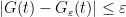
Proof: First suppose that converges in distribution to , and is continuous at . For any , one can find a such that

for every . One can also find an larger than such that and . Thus

and

Let be a continuous function supported on that equals on . Then by the above discussion we have

and hence

for large enough . In particular

A similar argument, replacing with a continuous function supported on that equals on gives

for large enough. Putting the two estimates together gives

for large enough; sending , we obtain the claim.
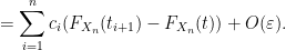
Conversely, suppose that converges to at every continuity point of . Let be a continuous compactly supported function, then it is uniformly continuous. As is monotone increasing, it can only have countably many points of discontinuity. From these two facts one can find, for any , a simple function for some that are points of continuity of , and real numbers , such that for all . Thus

Similarly for replaced by . Subtracting and taking limit superior, we conclude that

and on sending , we obtain that converges in distribution to as claimed.
The restriction to continuity points of is necessary. Consider for instance the deterministic random variables , then converges almost surely (and hence in distribution) to , but does not converge to .

Example 5 For any natural number , let be a discrete random variable drawn uniformly from the finite set , and let be the continuous random variable drawn uniformly from . Then converges in distribution to . Thus we see that a continuous random variable can emerge as the limit of discrete random variables.

Example 6 For any natural number , let be a continuous random variable drawn uniformly from , then converges in distribution to the deterministic real number . Thus we see that discrete (or even deterministic) random variables can emerge as the limit of continuous random variables.

Exercise 7 (Portmanteau theorem) Show that the properties (i) and (ii) in Proposition 4 are also equivalent to the following three statements:

• (iii) One has for all closed sets .
• (iv) One has for all open sets .
• (v) For any Borel set whose topological boundary is such that , one has .

(Note: to prove this theorem, you may wish to invoke Urysohn’s lemma. To deduce (iii) from (i), you may wish to start with the case of compact .)

We can now state the famous central limit theorem:

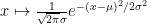
Theorem 8 (Central limit theorem) Let be iid copies of a scalar random variable of finite mean and finite non-zero variance . Let . Then the random variables converges in distribution to a random variable with the standard normal distribution (that is to say, a random variable with probability density function ). Thus, by abuse of notation

In the normalised case when has mean zero and unit variance, this simplifies to

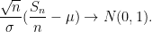
Using Proposition 4 (and the fact that the cumulative distribution function associated to is continuous, the central limit theorem is equivalent to asserting that

as for any , or equivalently that

Informally, one can think of the central limit theorem as asserting that approximately behaves like it has distribution for large , where is the normal distribution with mean and variance , that is to say the distribution with probability density function . The integrals can be written in terms of the error function as .
The central limit theorem is a basic example of the universality phenomenon in probability – many statistics involving a large system of many independent (or weakly dependent) variables (such as the normalised sums ) end up having a universal asymptotic limit (in this case, the normal distribution), regardless of the precise makeup of the underlying random variable that comprised that system. Indeed, the universality of the normal distribution is such that it arises in many other contexts than the fluctuation of iid random variables; the central limit theorem is merely the first place in probability theory where it makes a prominent appearance.

We will give several proofs of the central limit theorem in these notes; each of these proofs has their advantages and disadvantages, and can each extend to prove many further results beyond the central limit theorem. We first give Lindeberg’s proof of the central limit theorem, based on exchanging (or swapping) each component of the sum in turn. This proof gives an accessible explanation as to why there should be a universal limit for the central limit theorem; one then computes directly with gaussians to verify that it is the normal distribution which is the universal limit. Our second proof is the most popular one taught in probability texts, namely the Fourier-analytic proof based around the concept of the characteristic function of a real random variable . Thanks to the powerful identities and other results of Fourier analysis, this gives a quite short and direct proof of the central limit theorem, although the arguments may seem rather magical to readers who are not already familiar with Fourier methods. Finally, we give a proof based on the moment method, in the spirit of the arguments in the previous notes; this argument is more combinatorial, but is straightforward and is particularly robust, in particular being well equipped to handle some dependencies between components; we will illustrate this by proving the Erdos-Kac law in number theory by this method. Some further discussion of the central limit theorem (including some further proofs, such as one based on Stein’s method) can be found in this blog post. Some further variants of the central limit theorem, such as local limit theorems, stable laws, and large deviation inequalities, will be discussed in the next (and final) set of notes.

The following exercise illustrates the power of the central limit theorem, by establishing combinatorial estimates which would otherwise require the use of Stirling’s formula to establish.

Exercise 9 (De Moivre-Laplace theorem) Let be a Bernoulli random variable, taking values in with , thus has mean and variance . Let be iid copies of , and write .

• (i) Show that takes values in with . (This is an example of a binomial distribution.)
• (ii) Assume Stirling’s formula

  

  where is a function of that goes to zero as . (A proof of this formula may be found in this previous blog post.) Using this formula, and without using the central limit theorem, show that

  

  as for any fixed real numbers .

The above special case of the central limit theorem was first established by de Moivre and Laplace.

We close this section with some basic facts about convergence of distribution that will be useful in the sequel.

Exercise 10 Let , be sequences of real random variables, and let be further real random variables.

• (i) If is deterministic, show that converges in distribution to if and only if converges in probability to .
• (ii) Suppose that is independent of for each , and independent of . Show that converges in distribution to if and only if converges in distribution to and converges in distribution to . (The shortest way to prove this is by invoking the Stone-Weierstrass theorem, but one can also proceed by proving some version of Proposition 4.) What happens if the independence hypothesis is dropped?
• (iii) If converges in distribution to , show that for every there exists such that for all sufficiently large . (That is to say, is a tight sequence of random variables.)
• (iv) Show that converges in distribution to if and only if, after extending the probability space model if necessary, one can find copies and of and respectively such that converges almost surely to . (Hint: use the Skorohod representation, Exercise 29 of Notes 0.)
• (v) If converges in distribution to , and is continuous, show that converges in distribution to . Generalise this claim to the case when takes values in an arbitrary locally compact Hausdorff space.
• (vi) (Slutsky’s theorem) If converges in distribution to , and converges in probability to a deterministic limit , show that converges in distribution to , and converges in distribution to . (Hint: either use (iv), or else use (iii) to control some error terms.) This statement combines particularly well with (i). What happens if is not assumed to be deterministic?
• (vii) (Fatou lemma) If is continuous, and converges in distribution to , show that .
• (viii) (Bounded convergence) If is continuous and bounded, and converges in distribution to , show that .
• (ix) (Dominated convergence) If converges in distribution to , and there is an absolutely integrable such that almost surely for all , show that .

For future reference we also mention (but will not prove) Prokhorov’s theorem that gives a partial converse to part (iii) of the above exercise:

Theorem 11 (Prokhorov’s theorem) Let be a sequence of real random variables which is tight (that is, for every there exists such that for all sufficiently large ). Then there exists a subsequence which converges in distribution to some random variable (which may possibly be modeled by a different probability space model than the .)

The proof of this theorem relies on the Riesz representation theorem, and is beyond the scope of this course; but see for instance Exercise 29 of this previous blog post. (See also the closely related Helly selection theorem, covered in Exercise 30 of the same post.)