A generalized Cauchy-Schwarz inequality via the Gibbs variational formula

Let be a non-empty finite set. If is a random variable taking values in , the Shannon entropy of is defined as

There is a nice variational formula that lets one compute logs of sums of exponentials in terms of this entropy:

Lemma 1 (Gibbs variational formula) Let be a function. Then

Proof: Note that shifting by a constant affects both sides of (1) the same way, so we may normalize . Then is now the probability distribution of some random variable , and the inequality can be rewritten as

But this is precisely the Gibbs inequality. (The expression inside the supremum can also be written as , where denotes Kullback-Leibler divergence. One can also interpret this inequality as a special case of the Fenchel–Young inequality relating the conjugate convex functions and .)

In this note I would like to use this variational formula (which is also known as the Donsker-Varadhan variational formula) to give another proof of the following inequality of Carbery.

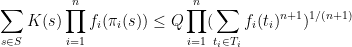
Theorem 2 (Generalized Cauchy-Schwarz inequality) Let , let be finite non-empty sets, and let be functions for each . Let and be positive functions for each . Then

where is the quantity

where is the set of all tuples such that for .

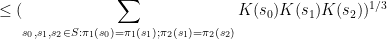
Thus for instance, the identity is trivial for . When , the inequality reads

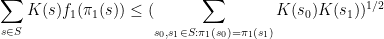
which is easily proven by Cauchy-Schwarz, while for the inequality reads

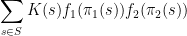
which can also be proven by elementary means. However even for , the existing proofs require the “tensor power trick” in order to reduce to the case when the are step functions (in which case the inequality can be proven elementarily, as discussed in the above paper of Carbery).

We now prove this inequality. We write and for some functions and . If we take logarithms in the inequality to be proven and apply Lemma 1, the inequality becomes

where ranges over random variables taking values in , range over tuples of random variables taking values in , and range over random variables taking values in . Comparing the suprema, the claim now reduces to

Lemma 3 (Conditional expectation computation) Let be an -valued random variable. Then there exists a -valued random variable , where each has the same distribution as , and

Proof: We induct on . When we just take . Now suppose that , and the claim has already been proven for , thus one has already obtained a tuple with each having the same distribution as , and

By hypothesis, has the same distribution as . For each value attained by , we can take conditionally independent copies of and conditioned to the events and respectively, and then concatenate them to form a tuple in , with a further copy of that is conditionally independent of relative to . One can the use the entropy chain rule to compute

and the claim now follows from the induction hypothesis.

With a little more effort, one can replace by a more general measure space (and use differential entropy in place of Shannon entropy), to recover Carbery’s inequality in full generality; we leave the details to the interested reader.

When is correlation transitive?

Given two unit vectors in a real inner product space, one can define the correlation between these vectors to be their inner product , or in more geometric terms, the cosine of the angle subtended by and . By the Cauchy-Schwarz inequality, this is a quantity between and , with the extreme positive correlation occurring when are identical, the extreme negative correlation occurring when are diametrically opposite, and the zero correlation occurring when are orthogonal. This notion is closely related to the notion of correlation between two non-constant square-integrable real-valued random variables , which is the same as the correlation between two unit vectors lying in the Hilbert space of square-integrable random variables, with being the normalisation of defined by subtracting off the mean and then dividing by the standard deviation of , and similarly for and .

One can also define correlation for complex (Hermitian) inner product spaces by taking the real part of the complex inner product to recover a real inner product.

While reading the (highly recommended) recent popular maths book “How not to be wrong“, by my friend and co-author Jordan Ellenberg, I came across the (important) point that correlation is not necessarily transitive: if correlates with , and correlates with , then this does not imply that correlates with . A simple geometric example is provided by the three unit vectors

in the Euclidean plane : and have a positive correlation of , as does and , but and are not correlated with each other. Or: for a typical undergraduate course, it is generally true that good exam scores are correlated with a deep understanding of the course material, and memorising from flash cards are correlated with good exam scores, but this does not imply that memorising flash cards is correlated with deep understanding of the course material.

However, there are at least two situations in which some partial version of transitivity of correlation can be recovered. The first is in the “99%” regime in which the correlations are very close to : if are unit vectors such that is very highly correlated with , and is very highly correlated with , then this does imply that is very highly correlated with . Indeed, from the identity

(and similarly for and ) and the triangle inequality

we see that

Thus, for instance, if and , then . This is of course closely related to (though slightly weaker than) the triangle inequality for angles:

Remark 1 (Thanks to Andrew Granville for conversations leading to this observation.) The inequality (1) also holds for sub-unit vectors, i.e. vectors with . This comes by extending in directions orthogonal to all three original vectors and to each other in order to make them unit vectors, enlarging the ambient Hilbert space if necessary. More concretely, one can apply (1) to the unit vectors

in .

But even in the “” regime in which correlations are very weak, there is still a version of transitivity of correlation, known as the van der Corput lemma, which basically asserts that if a unit vector is correlated with many unit vectors , then many of the pairs will then be correlated with each other. Indeed, from the Cauchy-Schwarz inequality

we see that

Thus, for instance, if for at least values of , then (after removing those indices for which ) must be at least , which implies that for at least pairs . Or as another example: if a random variable exhibits at least positive correlation with other random variables , then if , at least two distinct must have positive correlation with each other (although this argument does not tell you which pair are so correlated). Thus one can view this inequality as a sort of `pigeonhole principle” for correlation.

A similar argument (multiplying each by an appropriate sign ) shows the related van der Corput inequality

and this inequality is also true for complex inner product spaces. (Also, the do not need to be unit vectors for this inequality to hold.)

Geometrically, the picture is this: if positively correlates with all of the , then the are all squashed into a somewhat narrow cone centred at . The cone is still wide enough to allow a few pairs to be orthogonal (or even negatively correlated) with each other, but (when is large enough) it is not wide enough to allow all of the to be so widely separated. Remarkably, the bound here does not depend on the dimension of the ambient inner product space; while increasing the number of dimensions should in principle add more “room” to the cone, this effect is counteracted by the fact that in high dimensions, almost all pairs of vectors are close to orthogonal, and the exceptional pairs that are even weakly correlated to each other become exponentially rare. (See this previous blog post for some related discussion; in particular, Lemma 2 from that post is closely related to the van der Corput inequality presented here.)

A particularly common special case of the van der Corput inequality arises when is a unit vector fixed by some unitary operator , and the are shifts of a single unit vector . In this case, the inner products are all equal, and we arrive at the useful van der Corput inequality

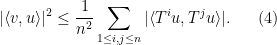
(In fact, one can even remove the absolute values from the right-hand side, by using (2) instead of (4).) Thus, to show that has negligible correlation with , it suffices to show that the shifts of have negligible correlation with each other.

Here is a basic application of the van der Corput inequality:

Proposition 2 (Weyl equidistribution estimate) Let be a polynomial with at least one non-constant coefficient irrational. Then one has

where .

Note that this assertion implies the more general assertion

for any non-zero integer (simply by replacing by ), which by the Weyl equidistribution criterion is equivalent to the sequence being asymptotically equidistributed in .

Proof: We induct on the degree of the polynomial , which must be at least one. If is equal to one, the claim is easily established from the geometric series formula, so suppose that and that the claim has already been proven for . If the top coefficient of is rational, say , then by partitioning the natural numbers into residue classes modulo , we see that the claim follows from the induction hypothesis; so we may assume that the top coefficient is irrational.

In order to use the van der Corput inequality as stated above (i.e. in the formalism of inner product spaces) we will need a non-principal ultrafilter (see e.g this previous blog post for basic theory of ultrafilters); we leave it as an exercise to the reader to figure out how to present the argument below without the use of ultrafilters (or similar devices, such as Banach limits). The ultrafilter defines an inner product on bounded complex sequences by setting

Strictly speaking, this inner product is only positive semi-definite rather than positive definite, but one can quotient out by the null vectors to obtain a positive-definite inner product. To establish the claim, it will suffice to show that

for every non-principal ultrafilter .

Note that the space of bounded sequences (modulo null vectors) admits a shift , defined by

This shift becomes unitary once we quotient out by null vectors, and the constant sequence is clearly a unit vector that is invariant with respect to the shift. So by the van der Corput inequality, we have

for any . But we may rewrite . Then observe that if , is a polynomial of degree whose coefficient is irrational, so by induction hypothesis we have for . For we of course have , and so

for any . Letting , we obtain the claim.

Estimation of the Type III sums

This is the final continuation of the online reading seminar of Zhang’s paper for the polymath8 project. (There are two other continuations; this previous post, which deals with the combinatorial aspects of the second part of Zhang’s paper, and this previous post, that covers the Type I and Type II sums.) The main purpose of this post is to present (and hopefully, to improve upon) the treatment of the final and most innovative of the key estimates in Zhang’s paper, namely the Type III estimate.

The main estimate was already stated as Theorem 17 in the previous post, but we quickly recall the relevant definitions here. As in other posts, we always take to be a parameter going off to infinity, with the usual asymptotic notation associated to this parameter.

Definition 1 (Coefficient sequences) A coefficient sequence is a finitely supported sequence that obeys the bounds

for all , where is the divisor function.

• (i) If is a coefficient sequence and is a primitive residue class, the (signed) discrepancy of in the sequence is defined to be the quantity

  

• (ii) A coefficient sequence is said to be at scale for some if it is supported on an interval of the form .
• (iii) A coefficient sequence at scale is said to be smooth if it takes the form for some smooth function supported on obeying the derivative bounds

  

  for all fixed (note that the implied constant in the notation may depend on ).

For any , let denote the square-free numbers whose prime factors lie in . The main result of this post is then the following result of Zhang:

Theorem 2 (Type III estimate) Let be fixed quantities, and let be quantities such that

and

and

for some fixed . Let be coefficient sequences at scale respectively with smooth. Then for any we have

In fact we have the stronger “pointwise” estimate

for all with and all , and some fixed .

(This is very slightly stronger than previously claimed, in that the condition has been dropped.)

It turns out that Zhang does not exploit any averaging of the factor, and matters reduce to the following:

Theorem 3 (Type III estimate without ) Let be fixed, and let be quantities such that

and

and

for some fixed . Let be smooth coefficient sequences at scales respectively. Then we have

for all and some fixed .

Let us quickly see how Theorem 3 implies Theorem 2. To show (4), it suffices to establish the bound

for all , where denotes a quantity that is independent of (but can depend on other quantities such as ). The left-hand side can be rewritten as

From Theorem 3 we have

where the quantity does not depend on or . Inserting this asymptotic and using crude bounds on (see Lemma 8 of this previous post) we conclude (4) as required (after modifying slightly).

It remains to establish Theorem 3. This is done by a set of tools similar to that used to control the Type I and Type II sums:

• (i) completion of sums;
• (ii) the Weil conjectures and bounds on Ramanujan sums;
• (iii) factorisation of smooth moduli ;
• (iv) the Cauchy-Schwarz and triangle inequalities (Weyl differencing).

The specifics are slightly different though. For the Type I and Type II sums, it was the classical Weil bound on Kloosterman sums that were the key source of power saving; Ramanujan sums only played a minor role, controlling a secondary error term. For the Type III sums, one needs a significantly deeper consequence of the Weil conjectures, namely the estimate of Bombieri and Birch on a three-dimensional variant of a Kloosterman sum. Furthermore, the Ramanujan sums – which are a rare example of sums that actually exhibit better than square root cancellation, thus going beyond even what the Weil conjectures can offer – make a crucial appearance, when combined with the factorisation of the smooth modulus (this new argument is arguably the most original and interesting contribution of Zhang).

A Fourier-free proof of the Furstenberg-Sarkozy theorem

The following result is due independently to Furstenberg and to Sarkozy:

Theorem 1 (Furstenberg-Sarkozy theorem) Let , and suppose that is sufficiently large depending on . Then every subset of of density at least contains a pair for some natural numbers with .

This theorem is of course similar in spirit to results such as Roth’s theorem or Szemerédi’s theorem, in which the pattern is replaced by or for some fixed respectively. There are by now many proofs of this theorem (see this recent paper of Lyall for a survey), but most proofs involve some form of Fourier analysis (or spectral theory). This may be compared with the standard proof of Roth’s theorem, which combines some Fourier analysis with what is now known as the density increment argument.

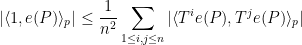
A few years ago, Ben Green, Tamar Ziegler, and myself observed that it is possible to prove the Furstenberg-Sarkozy theorem by just using the Cauchy-Schwarz inequality (or van der Corput lemma) and the density increment argument, removing all invocations of Fourier analysis, and instead relying on Cauchy-Schwarz to linearise the quadratic shift . As such, this theorem can be considered as even more elementary than Roth’s theorem (and its proof can be viewed as a toy model for the proof of Roth’s theorem). We ended up not doing too much with this observation, so decided to share it here.

The first step is to use the density increment argument that goes back to Roth. For any , let denote the assertion that for sufficiently large, all sets of density at least contain a pair with non-zero. Note that is vacuously true for . We will show that for any , one has the implication

for some absolute constant . This implies that is true for any (as can be seen by considering the infimum of all for which holds), which gives Theorem 1.

It remains to establish the implication (1). Suppose for sake of contradiction that we can find for which holds (for some sufficiently small absolute constant ), but fails. Thus, we can find arbitrarily large , and subsets of of density at least , such that contains no patterns of the form with non-zero. In particular, we have

(The exact ranges of and are not too important here, and could be replaced by various other small powers of if desired.)

Let be the density of , so that . Observe that

and

If we thus set , then

In particular, for large enough,

On the other hand, one easily sees that

and hence by the Cauchy-Schwarz inequality

which we can rearrange as

Shifting by we obtain (again for large enough)

In particular, by the pigeonhole principle (and deleting the diagonal case , which we can do for large enough) we can find distinct such that

so in particular

If we set and shift by , we can simplify this (again for large enough) as

On the other hand, since

we have

for any , and thus

Averaging this with (2) we conclude that

In particular, by the pigeonhole principle we can find such that

or equivalently has density at least on the arithmetic progression , which has length and spacing , for some absolute constant . By partitioning this progression into subprogressions of spacing and length (plus an error set of size , we see from the pigeonhole principle that we can find a progression of length and spacing on which has density at least (and hence at least ) for some absolute constant . If we then apply the induction hypothesis to the set

we conclude (for large enough) that contains a pair for some natural numbers with non-zero. This implies that lie in , a contradiction, establishing the implication (1).

A more careful analysis of the above argument reveals a more quantitative version of Theorem 1: for (say), any subset of of density at least for some sufficiently large absolute constant contains a pair with non-zero. This is not the best bound known; a (difficult) result of Pintz, Steiger, and Szemeredi allows the density to be as low as . On the other hand, this already improves on the (simpler) Fourier-analytic argument of Green that works for densities at least (although the original argument of Sarkozy, which is a little more intricate, works up to ). In the other direction, a construction of Rusza gives a set of density without any pairs .

Remark 1 A similar argument also applies with replaced by for fixed , because this sort of pattern is preserved by affine dilations into arithmetic progressions whose spacing is a power. By re-introducing Fourier analysis, one can also perform an argument of this type for where is the sum of two squares; see the above-mentioned paper of Green for details. However there seems to be some technical difficulty in extending it to patterns of the form for polynomials that consist of more than a single monomial (and with the normalisation , to avoid local obstructions), because one no longer has this preservation property.

Mixing for progressions in non-abelian groups

I’ve just uploaded to the arXiv my paper “Mixing for progressions in non-abelian groups“, submitted to Forum of Mathematics, Sigma (which, along with sister publication Forum of Mathematics, Pi, has just opened up its online submission system). This paper is loosely related in subject topic to my two previous papers on polynomial expansion and on recurrence in quasirandom groups (with Vitaly Bergelson), although the methods here are rather different from those in those two papers. The starting motivation for this paper was a question posed in this foundational paper of Tim Gowers on quasirandom groups. In that paper, Gowers showed (among other things) that if was a quasirandom group, patterns such as were mixing in the sense that, for any four sets , the number of such quadruples in was equal to , where , and denotes a quantity that goes to zero as the quasirandomness of the group goes to infinity. In my recent paper with Vitaly, we also considered mixing properties of some other patterns, namely and . This paper is concerned instead with the pattern , that is to say a geometric progression of length three. As observed by Gowers, by applying (a suitably quantitative version of) Roth’s theorem in (cosets of) a cyclic group, one can obtain a recurrence theorem for this pattern without much effort: if is an arbitrary finite group, and is a subset of with , then there are at least pairs such that , where is a quantity depending only on . However, this argument does not settle the question of whether there is a stronger mixing property, in that the number of pairs such that should be for any . Informally, this would assert that for chosen uniformly at random from , the triplet should resemble a uniformly selected element of in some weak sense.

For non-quasirandom groups, such mixing properties can certainly fail. For instance, if is the cyclic group (which is abelian and thus highly non-quasirandom) with the additive group operation, and for some small but fixed , then in the limit , but the number of pairs with is rather than . The problem here is that the identity ensures that if and both lie in , then has a highly elevated likelihood of also falling in . One can view as the preimage of a small ball under the one-dimensional representation defined by ; similar obstructions to mixing can also be constructed from other low-dimensional representations.

However, by definition, quasirandom groups do not have low-dimensional representations, and Gowers asked whether mixing for could hold for quasirandom groups. I do not know if this is the case for arbitrary quasirandom groups, but I was able to settle the question for a specific class of quasirandom groups, namely the special linear groups over a finite field in the regime where the dimension is bounded (but is at least two) and is large. Indeed, for such groups I can obtain a count of for the number of pairs with . In fact, I have the somewhat stronger statement that there are pairs with for any .

I was also able to obtain a partial result for the length four progression in the simpler two-dimensional case , but I had to make the unusual restriction that the group element was hyperbolic in the sense that it was diagonalisable over the finite field (as opposed to diagonalisable over the algebraic closure of that field); this amounts to the discriminant of the matrix being a quadratic residue, and this holds for approximately half of the elements of . The result is then that for any , one has pairs with hyperbolic and . (Again, I actually show a slightly stronger statement in which is restricted to an arbitrary subset of hyperbolic elements.)

For the length three argument, the main tools used are the Cauchy-Schwarz inequality, the quasirandomness of , and some algebraic geometry to ensure that a certain family of probability measures on that are defined algebraically are approximately uniformly distributed. The length four argument is significantly more difficult and relies on a rather ad hoc argument involving, among other things, expander properties related to the work of Bourgain and Gamburd, and also a “twisted” version of an argument of Gowers that is used (among other things) to establish an inverse theorem for the norm.

I give some details of these arguments below the fold.

Tricks Wiki: Use basic examples to calibrate exponents

Title: Use basic examples to calibrate exponents

Motivation: In the more quantitative areas of mathematics, such as analysis and combinatorics, one has to frequently keep track of a large number of exponents in one’s identities, inequalities, and estimates.  For instance, if one is studying a set of N elements, then many expressions that one is faced with will often involve some power of N; if one is instead studying a function f on a measure space X, then perhaps it is an norm which will appear instead.  The exponent involved will typically evolve slowly over the course of the argument, as various algebraic or analytic manipulations are applied.  In some cases, the exact value of this exponent is immaterial, but at other times it is crucial to have the correct value of at hand.   One can (and should) of course carefully go through one’s arguments line by line to work out the exponents correctly, but it is all too easy to make a sign error or other mis-step at one of the lines, causing all the exponents on subsequent lines to be incorrect.  However, one can guard against this (and avoid some tedious line-by-line exponent checking) by continually calibrating these exponents at key junctures of the arguments by using basic examples of the object of study (sets, functions, graphs, etc.) as test cases.  This is a simple trick, but it lets one avoid many unforced errors with exponents, and also lets one compute more rapidly.

Quick description: When trying to quickly work out what an exponent p in an estimate, identity, or inequality should be without deriving that statement line-by-line, test that statement with a simple example which has non-trivial behaviour with respect to that exponent p, but trivial behaviour with respect to as many other components of that statement as one is able to manage.   The “non-trivial” behaviour should be parametrised by some very large or very small parameter.  By matching the dependence on this parameter on both sides of the estimate, identity, or inequality, one should recover p (or at least a good prediction as to what p should be).

General discussion: The test examples should be as basic as possible; ideally they should have trivial behaviour in all aspects except for one feature that relates to the exponent p that one is trying to calibrate, thus being only “barely” non-trivial.   When the object of study is a function, then (appropriately rescaled, or otherwise modified) bump functions are very typical test objects, as are Dirac masses, constant functions, Gaussians, or other functions that are simple and easy to compute with.  In additive combinatorics, when the object of study is a subset of a group, then subgroups, arithmetic progressions, or random sets are typical test objects.  In graph theory, typical examples of test objects include complete graphs, complete bipartite graphs, and random graphs. And so forth.

This trick is closely related to that of using dimensional analysis to recover exponents; indeed, one can view dimensional analysis as the special case of exponent calibration when using test objects which are non-trivial in one dimensional aspect (e.g. they exist at a single very large or very small length scale) but are otherwise of a trivial or “featureless” nature.   But the calibration trick is more general, as it can involve parameters (such as probabilities, angles, or eccentricities) which are not commonly associated with the physical concept of a dimension.  And personally, I find example-based calibration to be a much more satisfying (and convincing) explanation of an exponent than a calibration arising from formal dimensional analysis.

When one is trying to calibrate an inequality or estimate, one should try to pick a basic example which one expects to saturate that inequality or estimate, i.e. an example for which the inequality is close to being an equality.  Otherwise, one would only expect to obtain some partial information on the desired exponent p (e.g. a lower bound or an upper bound only).  Knowing the examples that saturate an estimate that one is trying to prove is also useful for several other reasons – for instance, it strongly suggests that any technique which is not efficient when applied to the saturating example, is unlikely to be strong enough to prove the estimate in general, thus eliminating fruitless approaches to a problem and (hopefully) refocusing one’s attention on those strategies which actually have a chance of working.

Calibration is best used for the type of quick-and-dirty calculations one uses when trying to rapidly map out an argument that one has roughly worked out already, but without precise details; in particular, I find it particularly useful when writing up a rapid prototype.  When the time comes to write out the paper in full detail, then of course one should instead carefully work things out line by line, but if all goes well, the exponents obtained in that process should match up with the preliminary guesses for those exponents obtained by calibration, which adds confidence that there are no exponent errors have been committed.

Prerequisites: Undergraduate analysis and combinatorics.

The van der Corput trick, and equidistribution on nilmanifolds

This week I was in Columbus, Ohio, attending a conference on equidistribution on manifolds. I talked about my recent paper with Ben Green on the quantitative behaviour of polynomial sequences in nilmanifolds, which I have blogged about previously. During my talk (and inspired by the immediately preceding talk of Vitaly Bergelson), I stated explicitly for the first time a generalisation of the van der Corput trick which morally underlies our paper, though it is somewhat buried there as we specialised it to our application at hand (and also had to deal with various quantitative issues that made the presentation more complicated). After the talk, several people asked me for a more precise statement of this trick, so I am presenting it here, and as an application reproving an old theorem of Leon Green that gives a necessary and sufficient condition as to whether a linear sequence on a nilmanifold is equidistributed, which generalises the famous theorem of Weyl on equidistribution of polynomials.

UPDATE, Feb 2013: It has been pointed out to me by Pavel Zorin that this argument does not fully recover the theorem of Leon Green; to cover all cases, one needs the more complicated van der Corput argument in our paper.

254A, Lecture 12: Weakly mixing systems

In the previous lecture, we studied the recurrence properties of compact systems, which are systems in which all measurable functions exhibit almost periodicity – they almost return completely to themselves after repeated shifting. Now, we consider the opposite extreme of mixing systems – those in which all measurable functions (of mean zero) exhibit mixing – they become orthogonal to themselves after repeated shifting. (Actually, there are two different types of mixing, strong mixing and weak mixing, depending on whether the orthogonality occurs individually or on the average; it is the latter concept which is of more importance to the task of establishing the Furstenberg recurrence theorem.)

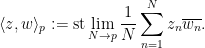
We shall see that for weakly mixing systems, averages such as can be computed very explicitly (in fact, this average converges to the constant ). More generally, we shall see that weakly mixing components of a system tend to average themselves out and thus become irrelevant when studying many types of ergodic averages. Our main tool here will be the humble Cauchy-Schwarz inequality, and in particular a certain consequence of it, known as the van der Corput lemma.

As one application of this theory, we will be able to establish Roth’s theorem (the k=3 case of Szemerédi’s theorem).