Operator splitting for the KdV equation

The summer continues to allow some clearing of the backlog of projects accumulated during the academic year: Helge Holden, Kenneth Karlsen, Nils Risebro, and myself have uploaded to the arXiv the paper “Operator splitting for the KdV equation“, submitted to Math. Comp..   This paper is concerned with accurate numerical schemes for solving initial value problems for the Korteweg-de Vries equation

(1)

though the analysis here would be valid for a wide range of other semilinear dispersive models as well.  In principle, these equations, which are completely integrable, can be solved exactly by the inverse scattering method, but fast and accurate implementations of this method are still not as satisfactory as one would like.  On the other hand, the linear Korteweg-de Vries equation

(2)

can be solved exactly (with accurate and fast numerics) via the (fast) Fourier transform, while the (inviscid) Burgers equation

(3)

can also be solved exactly (and quickly) by the method of characteristics.  Since the KdV equation is in some sense a combination of the equations (2) and (3), it is then reasonable to hope that some combination of the solution schemes for (2) and (3) can be used to solve (1), at least in some approximate sense.

One way to do this is by the method of operator splitting.  Observe from the formal approximation (where should be thought of as small, and is some matrix or linear operator), that one has

, (4)

[we do not assume A and B to commute here] and thus we formally have

(5)

if for some fixed time T (thus ).  As a consequence, if one wants to solve the linear ODE

(1′)

for time , one can achieve an approximate solution (accurate to order ) by alternating times between evolving the ODE

(2′)

for time , and evolving the ODE

(3′)

for time , starting with the initial data .

It turns out that this scheme can be formalised, and furthermore generalised to nonlinear settings such as those for the KdV equation (1).  More precisely, we show that if for some , then one can solve (1) to accuracy in norm for any fixed time by alternating between evolving (2) and (3) for times (this scheme is known as Godunov splitting).

Actually, one can obtain faster convergence by modifying the scheme, at the cost of requiring higher regularity on the data; the situation is similar to that of numerical integration (or quadrature), in which the midpoint rule or Simpson’s rule provide more accuracy than the Riemann integral if the integrand is smooth.  For instance, one has the variant

(6)

of (5), which can be seen by expansion to second order in (or by playing around with the Baker-Campbell-Hausdorff formula).  For KdV, we can rigorously show that the analogous scheme (known as Strang splitting) involving the indicated combination of evolutions of (2) and (3) will also converge to accuracy in norm, provided that and .

Bulk universality for Wigner hermitian matrices with subexponential decay

One further paper in this stream: László Erdős, José Ramírez, Benjamin Schlein, Van Vu, Horng-Tzer Yau, and myself have just uploaded to the arXiv the paper “Bulk universality for Wigner hermitian matrices with subexponential decay“, submitted to Mathematical Research Letters.  (Incidentally, this is my first six-author paper I have been involved in, not counting the polymath projects of course, though I have had a number of five-author papers.)

This short paper (9 pages) combines the machinery from two recent papers on the universality conjecture for the eigenvalue spacings in the bulk for Wigner random matrices (see my earlier blog post for more discussion).  On the one hand, the paper of Erdős-Ramírez-Schlein-Yau established this conjecture under the additional hypothesis that the distribution of the individual entries obeyed some smoothness and exponential decay conditions.  Meanwhile, the paper of Van Vu and myself (which I discussed in my earlier blog post) established the conjecture under a somewhat different set of hypotheses, namely that the distribution of the individual entries obeyed some moment conditions (in particular, the third moment had to vanish), a support condition (the entries had to have real part supported in at least three points), and an exponential decay condition.

After comparing our results, the six of us realised that our methods could in fact be combined rather easily to obtain a stronger result, establishing the universality conjecture assuming only a exponential decay (or more precisely, sub-exponential decay) bound on the coefficients; thus all regularity, moment, and support conditions have been eliminated.  (There is one catch, namely that we can no longer control a single spacing for a single fixed i, but must now average over all before recovering the universality.  This is an annoying technical issue but it may be resolvable in the future with further refinements to the method.)

I can describe the main idea behind the unified approach here.  One can arrange the Wigner matrices in a hierarchy, from most structured to least structured:

• The most structured (or special) ensemble is the Gaussian Unitary Ensemble (GUE), in which the coefficients are gaussian. Here, one has very explicit and tractable formulae for the eigenvalue distributions, gap spacing, etc.
• The next most structured ensemble of Wigner matrices are the Gaussian-divisible or Johansson matrices, which are matrices H of the form , where is another Wigner matrix, V is a GUE matrix independent of , and is a fixed parameter independent of n.  Here, one still has quite explicit (though not quite as tractable) formulae for the joint eigenvalue distribution and related statistics.  Note that the limiting case t=1 is GUE.
• After this, one has the Ornstein-Uhlenbeck-evolved matrices, which are also of the form , but now decays at a power rate with n, rather than being comparable to 1.  Explicit formulae still exist for these matrices, but extracting universality out of this is hard work (and occupies the bulk of the paper of Erdős-Ramírez-Schlein-Yau).
• Finally, one has arbitrary Wigner matrices, which can be viewed as the t=0 limit of the above Ornstein-Uhlenbeck process.

The arguments in the paper of Erdős-Ramírez-Schlein-Yau can be summarised as follows (I assume subexponential decay throughout this discussion):

1. (Structured case) The universality conjecture is true for Ornstein-Uhlenbeck-evolved matrices with for any .  (The case was treated in an earlier paper of Erdős-Ramírez-Schlein-Yau, while the case where t is comparable to 1 was treated by Johansson.)
2. (Matching) Every Wigner matrix with suitable smoothness conditions can be “matched” with an Ornstein-Uhlenbeck-evolved matrix, in the sense that the eigenvalue statistics for the two matrices are asymptotically identical.  (This is relatively easy due to the fact that can be taken arbitrarily close to zero.)
3. Combining 1. and 2. one obtains universality for all Wigner matrices obeying suitable smoothness conditions.

The arguments in the paper of Van and myself can be summarised as follows:

1. (Structured case) The universality conjecture is true for Johansson matrices, by the paper of Johansson.
2. (Matching) Every Wigner matrix with some moment and support conditions can be “matched” with a Johansson matrix, in the sense that the first four moments of the entries agree, and hence (by the Lindeberg strategy in our paper) have asymptotically identical statistics.
3. Combining 1. and 2. one obtains universality for all Wigner matrices obtaining suitable moment and support conditions.

What we realised is by combining the hard part 1. of the paper of Erdős-Ramírez-Schlein-Yau with the hard part 2. of the paper of Van and myself, we can remove all regularity, moment, and support conditions.  Roughly speaking, the unified argument proceeds as follows:

1. (Structured case) By the arguments of Erdős-Ramírez-Schlein-Yau, the universality conjecture is true for Ornstein-Uhlenbeck-evolved matrices with for any .
2. (Matching) Every Wigner matrix can be “matched” with an Ornstein-Uhlenbeck-evolved matrix for (say), in the sense that the first four moments of the entries almost agree, which is enough (by the arguments of Van and myself) to show that these two matrices have asymptotically identical statistics on the average.
3. Combining 1. and 2. one obtains universality for the averaged statistics for all Wigner matrices.

The averaging should be removable, but this would require better convergence results to the semicircular law than are currently known (except with additional hypotheses, such as vanishing third moment).  The subexponential decay should also be relaxed to a condition of finiteness for some fixed moment , but we did not pursue this direction in order to keep the paper short.

Sumset and inverse sumset theorems for Shannon entropy

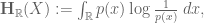
It turns out to be a favourable week or two for me to finally finish a number of papers that had been at a nearly completed stage for a while.  I have just uploaded to the arXiv my article “Sumset and inverse sumset theorems for Shannon entropy“, submitted to Combinatorics, Probability, and Computing.  This paper evolved from a “deleted scene” in my book with Van Vu entitled “Entropy sumset estimates“.  In those notes, we developed analogues of the standard Plünnecke-Ruzsa sumset estimates (which relate quantities such as the cardinalities of the sum and difference sets of two finite sets in an additive group to each other), to the entropy setting, in which the finite sets are replaced instead with discrete random variables taking values in that group G, and the (logarithm of the) cardinality |A| is replaced with the Shannon entropy

This quantity measures the information content of X; for instance, if , then it will take k bits on the average to store the value of X (thus a string of n independent copies of X will require about nk bits of storage in the asymptotic limit ).  The relationship between entropy and cardinality is that if X is the uniform distribution on a finite non-empty set A, then .  If instead X is non-uniformly distributed on A, one has , thanks to Jensen’s inequality.

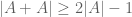
It turns out that many estimates on sumsets have entropy analogues, which resemble the “logarithm” of the sumset estimates.  For instance, the trivial bounds

have the entropy analogue

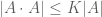
whenever X, Y are independent discrete random variables in an additive group; this is not difficult to deduce from standard entropy inequalities.  Slightly more non-trivially, the sum set estimate

established by Ruzsa, has an entropy analogue

,

and similarly for a number of other standard sumset inequalities in the literature (e.g. the Rusza triangle inequality, the Plünnecke-Rusza inequality, and the Balog-Szemeredi-Gowers theorem, though the entropy analogue of the latter requires a little bit of care to state).  These inequalities can actually be deduced fairly easily from elementary arithmetic identities, together with standard entropy inequalities, most notably the submodularity inequality

whenever X,Y,Z,W are discrete random variables such that X and Y each determine W separately (thus for some deterministic functions f, g) and X and Y determine Z jointly (thus for some deterministic function f).  For instance, if X,Y,Z are independent discrete random variables in an additive group G, then and each determine separately, and determine jointly, leading to the inequality

which soon leads to the entropy Rusza triangle inequality

which is an analogue of the combinatorial Ruzsa triangle inequality

All of this was already in the unpublished notes with Van, though I include it in this paper in order to place it in the literature.  The main novelty of the paper, though, is to consider the entropy analogue of Freiman’s theorem, which classifies those sets A for which .  Here, the analogous problem is to classify the random variables such that , where are independent copies of X.  Let us say that X has small doubling if this is the case.

For instance, the uniform distribution U on a finite subgroup H of G has small doubling (in fact in this case). In a similar spirit, the uniform distribution on a (generalised) arithmetic progression P also has small doubling, as does the uniform distribution on a coset progression H+P.  Also, if X has small doubling, and Y has bounded entropy, then X+Y also has small doubling, even if Y and X are not independent.  The main theorem is that these are the only cases:

Theorem 1. (Informal statement) X has small doubling if and only if for some uniform distribution U on a coset progression (of bounded rank), and Y has bounded entropy.

For instance, suppose that X was the uniform distribution on a dense subset A of a finite group G.  Then Theorem 1 asserts that X is close in a “transport metric” sense to the uniform distribution U on G, in the sense that it is possible to rearrange or transport the probability distribution of X to the probability distribution of U (or vice versa) by shifting each component of the mass of X by an amount Y which has bounded entropy (which basically means that it primarily ranges inside a set of bounded cardinality).  The way one shows this is by randomly translating the mass of X around by a few random shifts to approximately uniformise the distribution, and then deal with the residual fluctuation in the distribution by hand.  Theorem 1 as a whole is established by using the Freiman theorem in the combinatorial setting combined with various elementary convexity and entropy inequality arguments to reduce matters to the above model case when X is supported inside a finite group G and has near-maximal entropy.

I also show a variant of the above statement: if X, Y are independent and , then we have (i.e. X has the same distribution as Y+Z for some Z of bounded entropy (not necessarily independent of X or Y).  Thus if two random variables are additively related to each other, then they can be additively transported to each other by using a bounded amount of entropy.

In the last part of the paper I relate these discrete entropies to their continuous counterparts

where X is now a continuous random variable on the real line with density function .  There are a number of sum set inequalities known in this setting, for instance

,

for independent copies of a finite entropy random variable X, with equality if and only if X is a Gaussian.  Using this inequality and Theorem 1, I show a discrete version, namely that

,

whenever and are independent copies of a random variable in (or any other torsion-free abelian group) whose entropy is sufficiently large depending on .  This is somewhat analogous to the classical sumset inequality

though notice that we have a gain of just rather than here, the point being that there is a Gaussian counterexample in the entropy setting which does not have a combinatorial analogue (except perhaps in the high-dimensional limit).  The main idea is to use Theorem 1 to trap most of X inside a coset progression, at which point one can use Fourier-analytic additive combinatorial tools to show that the distribution is “smooth” in some non-trivial direction r, which can then be used to approximate the discrete distribution by a continuous one.

I also conjecture more generally that the entropy monotonicity inequalities established by Artstein, Barthe, Ball, and Naor in the continuous case also hold in the above sense in the discrete case, though my method of proof breaks down because I no longer can assume small doubling.

Freiman’s theorem for solvable groups

I’m continuing the stream of uploaded papers this week with my paper “Freiman’s theorem for solvable groups“, submitted to Contrib. Disc. Math..  This paper concerns the problem (discussed in this earlier blog post) of determining the correct analogue of Freiman’s theorem in a general non-abelian group .  Specifically, if is a finite set that obeys the doubling condition for some bounded K, what does this tell us about A?  Heuristically, we expect A to behave like a finite subgroup of G (or perhaps a coset of such a subgroup).

When G is the integers (with the additive group operation), Freiman’s theorem then tells us that A is controlled by a generalised arithmetic progression P, where I say that one set A is controlled by another P if they have comparable size, and the former can be covered by a finite number of translates of the latter.  (One can view generalised arithmetic progressions as an approximate version of a subgroup, in which one only uses the generators of the progression for a finite amount of time before stopping, as opposed to groups which allow words of unbounded length in the generators.) For more general abelian groups, the Freiman theorem of Green and Ruzsa tells us that a set of bounded doubling is controlled by a generalised coset progression , i.e. the sum of a generalised arithmetic progression P and a finite subgroup H of G.  (Of course, if G is torsion-free, the finite subgroup H must be trivial.)

In this paper we address the case when G is a solvable group of bounded derived length.  The main result is that if a subset of G has small doubing, then it is controlled by an object which I call a “coset nilprogression”, which is a certain technical generalisation of a coset progression, in which the generators do not quite commute, but have commutator expressible in terms of “higher order” generators.  This is essentially a sharp characterisation of such sets, except for the fact that one would like a more explicit description of these coset nilprogressions.   In the torsion-free case, a more explicit description (analogous to the Mal’cev basis description of nilpotent groups) has appeared in a very recent paper of Breulliard and Green; in the case of monomial groups (a class of groups that overlaps to a large extent with solvable groups), and assuming a polynomial growth condition rather than a doubling condition, a related result controlling A by balls in a suitable type of metric has appeared in very recent work of Sanders.  In the nilpotent case there is also a nice recent argument of Fisher, Peng, and Katz which shows that sets of small doubling remain of small doubling with respect to the Lie algebra operations of addition and Lie bracket, and thus are amenable to the abelian Freiman theorems.

The conclusion of my paper is easiest to state (and easiest to prove) in the model case of the lamplighter group , where is the additive group of doubly infinite sequences in the finite field with only finitely many non-zero entries, and acts on this space by translations.  This is a solvable group of derived length two.  The main result here is

Theorem 1. (Freiman’s theorem for the lamplighter group) If has bounded doubling, then A is controlled either by a finite subspace of the “vertical” group , or else by a set of the form , where is a generalised arithmetic progression, and obeys the Freiman isomorphism property whenever and .

This result, incidentally, recovers an earlier result of Lindenstrauss that the lamplighter group does not contain a Følner sequence of sets of uniformly bounded doubling.  It is a good exercise to establish the “exact” version of this theorem, in which one classifies subgroups of the lamplighter group rather than sets of small doubling; indeed, the proof of this the above theorem follows fairly closely the natural proof of the exact version.

One application of the solvable Freiman theorem is the following quantitative version of a classical result of Milnor and of Wolf, which asserts that any solvable group of polynomial growth is virtually nilpotent:

Theorem 2. (Quantitative Milnor-Wolf theorem) Let G be a solvable group of derived length O(1), let S be a set of generators for G, and suppose one has the polynomial growth condition for some d = O(1), where is the set of all words generated by S of length at most R.  If R is sufficiently large, then this implies that G is virtually nilpotent; more precisely, G contains a nilpotent subgroup of step O(1) and index .

The key points here are that one only needs polynomial growth at a single scale R, rather than on many scales, and that the index of the nilpotent subgroup has polynomial size.

The proofs are based on an induction on the derived length.  After some standard manipulations (basically, splitting A by an approximate version of a short exact sequence), the problem boils down to that of understanding the action of some finite set A on a set E in an additive group.  If one assumes that E has small doubling and that the action of A leaves E approximately invariant, then one can show that E is a coset progression, and the action of A can be described efficiently using the generators of that progression (after refining the set A a bit).

In the course of the proof we need two new additive combinatorial results which may be of independent interest.  The first is a variant of a well-known theorem of Sárközy, which asserts that if A is a large subset of an arithmetic progression P, then an iterated sumset kA of A for some itself contains a long arithmetic progression. Here, we need the related fact that if A is a large subset of a coset progression, then an iterated subset kA for contains a large coset progression Q, and furthermore this inclusion is “robust” in the sense that all elements the elements of Q have a large number of representations as sums of elements of A.  We also need a new (non-commutative) variant of the Balog-Szemerédi(-Gowers) lemma, which asserts that if A has small doubling, then A (or more precisely ) contains a large “core” subset D such that almost all of a large iterated subset kD of D still lies inside ).  (This may not look like the usual Balog-Szemerédi lemma, but the proof of the lemma is almost identical to the original proof of Balog and Szemerédi, in particular relying on the Szemerédi regularity lemma.

An equivalence between inverse sumset theorems and inverse conjectures for the U^3 norm

For a number of reasons, including the start of the summer break for me and my coauthors, a number of papers that we have been working on are being released this week.  For instance, Ben Green and I have just uploaded to the arXiv our paper “An equivalence between inverse sumset theorems and inverse conjectures for the norm“, submitted to Math. Proc. Camb. Phil. Soc..  The main result of this short paper (which was briefly announced in this earlier post) is a connection between two types of inverse theorems in additive combinatorics, namely the inverse sumset theorems of Freiman type, and inverse theorems for the Gowers uniformity norm, and more specifically, for the norm

on finite additive group G, where is a complex-valued function.

As usual, the connection is easiest to state in a finite field model such as .  In this case, we have the following inverse sumset theorem of Ruzsa:

Theorem 1. If is such that , then A can be covered by a translate of a subspace of of cardinality at most .

The constant has been improved for large in a sequence of papers, from by Ruzsa, by Green-Ruzsa, by Sanders, by Green and myself, and finally by Konyagin (private communication) which is sharp except for the precise value of the O() implied constant (as can be seen by considering the example when A consists of about 2K independent elements).  However, it is conjectured that the polynomial loss can be removed entirely if one modifies the conclusion slightly:

Conjecture 1. (Polynomial Freiman-Ruzsa conjecture for .) If is such that , then A can be covered by translates of subspaces of of cardinality at most |A|.

This conjecture was verified for downsets by Green and myself, but is open in general.   This conjecture has a number of equivalent formulations; see this paper of Green for more discussion.  In this previous post we show that a stronger version of this conjecture fails.

Meanwhile, for the Gowers norm, we have the following inverse theorem, due to Samorodnitsky:

Theorem 2. Let be a function whose norm is at least 1/K.  Then there exists a quadratic polynomial such that .

Note that the quadratic phases are the only functions taking values in [-1,1] whose norm attains its maximal value of 1.

It is conjectured that the exponentially weak correlation here can be strengthened to a polynomial one:

Conjecture 2. (Polynomial inverse conjecture for the norm). Let be a function whose norm is at least 1/K.  Then there exists a quadratic polynomial such that .

The first main result of this paper is

Theorem 3. Conjecture 1 and Conjecture 2 are equivalent.

This result was also independently observed by Shachar Lovett (private communication).  We also establish an analogous result for the cyclic group , in which the notion of polynomial is replaced by that of a subexponential , and in which the notion of a quadratic polynomial is replaced by a 2-step nilsequence; the precise statement is a bit technical and will not be given here.  We also observe a partial partial analogue of the correpsondence between inverse sumset theorems and Gowers norms in the higher order case, in particular observing that inverse theorems imply a certain rigidity result for “Freiman-quadratic polynomials” (a quadratic version of Conjecture 3 below).

Below the fold, we sketch the proof of Theorem 3.

Global regularity for a logarithmically supercritical hyperdissipative Navier-Stokes equation

I’ve just uploaded to the arXiv my paper “Global regularity for a logarithmically supercritical hyperdissipative Navier-Stokes equation“, submitted to Analysis & PDE.  It is a famous problem to establish the existence of global smooth solutions to the three-dimensional Navier-Stokes system of equations

given smooth, compactly supported, divergence-free initial data .

I do not claim to have any substantial progress on this problem here.  Instead, the paper makes a small observation about the hyper-dissipative version of the Navier-Stokes equations, namely

for some .  It is a folklore result that global regularity for this equation holds for ; the significance of the exponent is that it is energy-critical, in the sense that the scaling which preserves this particular hyper-dissipative Navier-Stokes equation, also preserves the energy.

Values of below (including, unfortunately, the case , which is the original Navier-Stokes equation) are supercritical and thus establishing global regularity beyond the reach of most known methods (see my earlier blog post for more discussion).

A few years ago, I observed (in the case of the spherically symmetric wave equation) that this “criticality barrier” had a very small amount of flexibility to it, in that one could push a critical argument to a slightly supercritical one by exploiting spacetime integral estimates a little bit more.  I realised recently that the same principle applied to hyperdissipative Navier-Stokes; here, the relevant spacetime integral estimate is the energy dissipation inequality

which ensures that the energy dissipation is locally integrable (and in fact globally integrable) in time.

In this paper I push the global regularity results by a fraction of a logarithm from towards .  For instance, the argument shows that the logarithmically supercritical equation

(0)

admits global smooth solutions.

The argument is in fact quite simple (the paper is seven pages in length), and relies on known technology; one just applies the energy method and a logarithmically modified Sobolev inequality in the spirit of a well-known inequality of Brezis and Wainger.  It looks like it will take quite a bit of effort though to improve the logarithmic factor much further.

One way to explain the tiny bit of wiggle room beyond the critical case is as follows.  The standard energy method approach to the critical Navier-Stokes equation relies at one stage on Gronwall’s inequality, which among other things asserts that if a time-dependent non-negative quantity E(t) obeys the differential inequality

(1)

and was locally integrable, then E does not blow up in time; in fact, one has the inequality

.

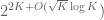
A slight modification of the argument shows that one can replace the linear inequality with a slightly superlinear inequality.  For instance, the differential inequality

(2)

also does not blow up in time; indeed, a separation of variables argument gives the explicit double-exponential bound

(let’s take and all functions smooth, to avoid technicalities).  It is this ability to go beyond Gronwall’s inequality by a little bit which is really at the heart of the logarithmically supercritical phenomenon.  In the paper, I establish an inequality basically of the shape (2), where is a suitably high-regularity Sobolev norm of , and is basically the energy dissipation mentioned earlier.  The point is that the logarithmic loss of in the dissipation can eventually be converted (by a Brezis-Wainger type argument) to a logarithmic loss in the high-regularity energy, as this energy can serve as a proxy for the frequency , which in turn serves as a proxy for the Laplacian .

To put it another way, with a linear exponential growth model, such as , it takes a constant amount of time for E to double, and so E never becomes infinite in finite time.  With an equation such as , the time taken for E to double from (say) to now shrinks to zero, but only as quickly as the harmonic series , so it still takes an infinite amount of time for E to blow up.  But because the divergence of is logarithmically slow, the growth of E is now a double exponential rather than a single one.  So there is a little bit of room to exploit between exponential growth and blowup.

Interestingly, there is a heuristic argument that suggests that the half-logarithmic loss in (0) can be widened to a full logarithmic loss, which I give below the fold.

Global regularity of wave maps VI. Abstract theory of minimal-energy blowup solutions

I’ve just uploaded to the arXiv my paper “Global regularity of wave maps VI.  Abstract theory of minimal-energy blowup solutions“, to be submitted with the rest of the “heatwave” project to establish global regularity (and scattering) for energy-critical wave maps into hyperbolic space.  Initially, this paper was intended to cap off the project by showing that if global regularity failed, then a special minimal energy blowup solution must exist, which enjoys a certain almost periodicity property modulo the symmetries of the equation.  However, the argument was more technical than I anticipated, and so I am splitting the paper into a relatively short high-level paper (this one) that reduces the problem to four smaller propositions, and a much longer technical paper which establishes those propositions, by developing a substantial amount of perturbation theory for wave maps.  I am pretty sure though that this process will not iterate any further, and paper VII will be my final paper in this series (and which I hope to finish by the end of this summer).  It is also worth noting that a number of papers establishing similar results (though with slightly different hypotheses and conclusions) will shortly appear by Sterbenz-Tataru and Krieger-Schlag.

Almost periodic minimal energy blowup solutions have been constructed for a variety of critical equations, such as the nonlinear Schrodinger equation (NLS) and the nonlinear wave equation (NLW).  The formal definition of almost periodicity is that the orbit of the solution stays in a precompact subset of the energy space once one quotients out by the non-compact symmetries of the equation (namely, translation and dilation).   Another (more informal) way of saying this is that for every time , there exists a position and a frequency such that the solution is localised in space in the region and in frequency in the region , with the solution decaying in energy away from these regions of space and frequency.  Model examples of almost periodic solutions include traveling waves (in which N(t) is fixed, and x(t) moves at constant velocity) and self-similar solutions (in which x(t) is fixed, and N(t) blows up in finite time at some power law rate).

Intuitively, the reason almost periodic minimal energy blowup solutions ought to exist in the absence of global regularity is as follows.  It is known (for any of the equations mentioned above) that global regularity (and scattering) holds at sufficiently small energies.  Thus, if global regularity fails at high energies, there must exist a critical energy , below which solutions exist globally (and obey scattering bounds), and above which solutions can blow up.

Now consider a solution at the critical energy which blows up (actually, for technical reasons, we instead consider a sequence of solutions approaching this critical energy which come increasingly close to blowing up, but let’s ignore this for now).  We claim that this solution must be localised in both space and frequency at every time, thus giving the desired almost periodic minimal energy blowup solution.  Indeed, suppose is not localised in frequency at some time t; then one can decompose into a high frequency component and a low frequency component , both of which have strictly smaller energy than , and which are widely separated from each other in frequency space.  By hypothesis, each of and can then be extended to global solutions, which should remain widely separated in frequency (because the linear analogues of these equations are constant-coefficient and thus preserve frequency support).   Assuming that interactions between very high and very low frequencies are negligible, this implies that the superposition approximately obeys the nonlinear equation; with a suitable perturbation theory, this implies that is close to .  But then is not blowing up, a contradiction.   The situation with spatial localisation is similar, but is somewhat more complicated due to the fact that spatial support, in contrast to frequency support, is not preserved by the linear evolution, let alone the nonlinear evolution.

As mentioned before, this type of scheme has been successfully implemented on a number of equations such as NLS and NLW.  However, there are two main obstacles in establishing it for wave maps.  The first is that the wave maps equation is not a scalar equation: the unknown field takes values in a target manifold (specifically, in a hyperbolic space) rather than in a Euclidean space.  As a consequence, it is not obvious how one would perform operations such as “decompose the solution into low frequency and high frequency components”, or the inverse operation “superimpose the low frequency and high frequency components to reconstitute the solution”.  Another way of viewing the problem is that the various component fields of the solution have to obey a number of important compatibility conditions which can be disrupted by an overly simple-minded approach to decomposition or reconstitution of solutions.

The second problem is that the interaction between very high and very low frequencies for wave maps turns out to not be entirely negligible: the high frequencies do have a negligible impact on the evolution of the low frequencies, but the low frequencies can “rotate” the high frequencies by acting as a sort of magnetic field (or more precisely, a connection) for the evolution of those high frequencies.  So the combined evolution of the high and low frequencies is not well approximated by a naive superposition of the separate evolutions of these frequency components.

DHJ: Still writing the second paper

This is a continuation of the previous thread here in the polymath1 project, which is now full.  Ostensibly, the purpose of this thread is to continue writing up the paper containing many of the things achieved during this side of the project, though we have also been spending time on chasing down more results, in particular using new computer data to narrow down the range of the maximal size of  6D Moser sets (currently we can pin this down to between 353 and 355).   At some point we have to decide what results to put in in full detail in the paper, what results to summarise only (with links to the wiki), and what results to defer to perhaps a subsequent paper, but these decisions can be taken at a leisurely pace.

I guess we’ve abandoned the numbering system now, but I suppose that if necessary we can use timestamps or URLs to link to previous comments.

The Szemerédi-Trotter theorem and the cell decomposition

The celebrated Szemerédi-Trotter theorem gives a bound for the set of incidences between a finite set of points and a finite set of lines in the Euclidean plane . Specifically, the bound is

where we use the asymptotic notation or to denote the statement that for some absolute constant . In particular, the number of incidences between points and lines is . This bound is sharp; consider for instance the discrete box with being the collection of lines . One easily verifies that , , and , showing that (1) is essentially sharp in the case ; one can concoct similar examples for other regimes of and .

On the other hand, if one replaces the Euclidean plane by a finite field geometry , where is a finite field, then the estimate (1) is false. For instance, if is the entire plane , and is the set of all lines in , then are both comparable to , but is comparable to , thus violating (1) when is large. Thus any proof of the Szemerédi-Trotter theorem must use a special property of the Euclidean plane which is not enjoyed by finite field geometries. In particular, this strongly suggests that one cannot rely purely on algebra and combinatorics to prove (1); one must also use some Euclidean geometry or topology as well.

Nowadays, the slickest proof of the Szemerédi-Trotter theorem is via the crossing number inequality (as discussed in this previous post), which ultimately relies on Euler’s famous formula ; thus in this argument it is topology which is the feature of Euclidean space which one is exploiting, and which is not present in the finite field setting. Today, though, I would like to mention a different proof (closer in spirit to the original proof of Szemerédi-Trotter, and also a later argument of Clarkson et al.), based on the method of cell decomposition, which has proven to be a very flexible method in combinatorial incidence geometry. Here, the distinctive feature of Euclidean geometry one is exploiting is convexity, which again has no finite field analogue.

Roughly speaking, the idea is this. Using nothing more than the axiom that two points determine at most one line, one can obtain the bound

which is inferior to (1). (On the other hand, this estimate works in both Euclidean and finite field geometries, and is sharp in the latter case, as shown by the example given earlier.) Dually, the axiom that two lines determine at most one point gives the bound

(or alternatively, one can use projective duality to interchange points and lines and deduce (3) from (2)).

An inspection of the proof of (2) shows that it is only expected to be sharp when the bushes associated to each point behave like “independent” subsets of , so that there is no significant correlation between the bush of one point and the bush of another point .

However, in Euclidean space, we have the phenomenon that the bush of a point is influenced by the region of space that lies in. Clearly, if lies in a set (e.g. a convex polygon), then the only lines that can contribute to are those lines which pass through . If is a small convex region of space, one expects only a fraction of the lines in to actually pass through . As such, if and both lie in , then and are compressed inside a smaller subset of , namely the set of lines passing through , and so should be more likely to intersect than if they were independent. This should lead to an improvement to (2) (and indeed, as we shall see below, ultimately leads to (1)).

More formally, the argument proceeds by applying the following lemma:

Lemma 1 (Cell decomposition) Let be a finite collection of lines in , let be a finite set of points, and let . Then it is possible to find a set of lines in , plus some additional open line segments not containing any point in , which subdivide into convex regions (or cells), such that the interior of each such cell is incident to at most lines.

The deduction of (1) from (2), (3) and Lemma 1 is very quick. Firstly we may assume we are in the range

otherwise the bound (1) follows already from either (2) or (3) and some high-school algebra.

Let be a parameter to be optimised later. We apply the cell decomposition to subdivide into open convex regions, plus a family of lines. Each of the convex regions has only lines through it, and so by (2) contributes incidences. Meanwhile, on each of the lines in used to perform this decomposition, there are at most transverse incidences (because each line in distinct from can intersect at most once), plus all the incidences along itself. Putting all this together, one obtains

We optimise this by selecting ; from (4) we can ensure that , so that . One then obtains

We can iterate away the error (halving the number of lines each time) and sum the resulting geometric series to obtain (1).

It remains to prove (1). If one subdivides using arbitrary lines, one creates at most cells (because each new line intersects the existing lines at most once, and so can create at most distinct cells), and for a similar reason, every line in visits at most of these regions, and so by double counting one expects lines per cell “on the average”. The key difficulty is then to get lines through every cell, not just on the average. It turns out that a probabilistic argument will almost work, but with a logarithmic loss (thus having lines per cell rather than ); but with a little more work one can then iterate away this loss also. The arguments here are loosely based on those of Clarkson et al.; a related (deterministic) decomposition also appears in the original paper of Szemerédi and Trotter. But I wish to focus here on the probabilistic approach.)

It is also worth noting that the original (somewhat complicated) argument of Szemerédi-Trotter has been adapted to establish the analogue of (1) in the complex plane by Toth, while the other known proofs of Szemerédi-Trotter, so far, have not been able to be extended to this setting (the Euler characteristic argument clearly breaks down, as does any proof based on using lines to divide planes into half-spaces). So all three proofs have their advantages and disadvantages.

Talagrand’s concentration inequality

In the theory of discrete random matrices (e.g. matrices whose entries are random signs ), one often encounters the problem of understanding the distribution of the random variable , where is an -dimensional random sign vector (so is uniformly distributed in the discrete cube ), and is some -dimensional subspace of for some .

It is not hard to compute the second moment of this random variable. Indeed, if denotes the orthogonal projection matrix from to the orthogonal complement of , then one observes that

and so upon taking expectations we see that

since is a rank orthogonal projection. So we expect to be about on the average.

In fact, one has sharp concentration around this value, in the sense that with high probability. More precisely, we have

Proposition 1 (Large deviation inequality) For any , one has

for some absolute constants .

In fact the constants are very civilised; for large one can basically take and , for instance. This type of concentration, particularly for subspaces of moderately large codimension , is fundamental to much of my work on random matrices with Van Vu, starting with our first paper (in which this proposition first appears). (For subspaces of small codimension (such as hyperplanes) one has to use other tools to get good results, such as inverse Littlewood-Offord theory or the Berry-Esséen central limit theorem, but that is another story.)

Proposition 1 is an easy consequence of the second moment computation and Talagrand’s inequality, which among other things provides a sharp concentration result for convex Lipschitz functions on the cube ; since is indeed a convex Lipschitz function, this inequality can be applied immediately. The proof of Talagrand’s inequality is short and can be found in several textbooks (e.g. Alon and Spencer), but I thought I would reproduce the argument here (specialised to the convex case), mostly to force myself to learn the proof properly. Note the concentration of obtained by Talagrand’s inequality is much stronger than what one would get from more elementary tools such as Azuma’s inequality or McDiarmid’s inequality, which would only give concentration of about or so (which is in fact trivial, since the cube has diameter ); the point is that Talagrand’s inequality is very effective at exploiting the convexity of the problem, as well as the Lipschitz nature of the function in all directions, whereas Azuma’s inequality can only easily take advantage of the Lipschitz nature of the function in coordinate directions. On the other hand, Azuma’s inequality works just as well if the metric is replaced with the larger metric, and one can conclude that the distance between and concentrates around its median to a width , which is a more non-trivial fact than the concentration bound given by that inequality. (The computation of the median of the distance is more complicated than for the distance, though, and depends on the orientation of .)

Remark 1 If one makes the coordinates of iid Gaussian variables rather than random signs, then Proposition 1 is much easier to prove; the probability distribution of a Gaussian vector is rotation-invariant, so one can rotate to be, say, , at which point is clearly the sum of independent squares of Gaussians (i.e. a chi-square distribution), and the claim follows from direct computation (or one can use the Chernoff inequality). The gaussian counterpart of Talagrand’s inequality is more classical, being essentially due to Lévy, and will also be discussed later in this post.