Conserved quantities for the Euler equations

The Euler equations for incompressible inviscid fluids may be written as

where is the velocity field, and is the pressure field. To avoid technicalities we will assume that both fields are smooth, and that is bounded. We will take the dimension to be at least two, with the three-dimensional case being of course especially interesting.

The Euler equations are the inviscid limit of the Navier-Stokes equations; as discussed in my previous post, one potential route to establishing finite time blowup for the latter equations when is to be able to construct “computers” solving the Euler equations, which generate smaller replicas of themselves in a noise-tolerant manner (as the viscosity term in the Navier-Stokes equation is to be viewed as perturbative noise).

Perhaps the most prominent obstacles to this route are the conservation laws for the Euler equations, which limit the types of final states that a putative computer could reach from a given initial state. Most famously, we have the conservation of energy

 

(assuming sufficient decay of the velocity field at infinity); thus for instance it would not be possible for a computer to generate a replica of itself which had greater total energy than the initial computer. This by itself is not a fatal obstruction (in this paper of mine, I constructed such a “computer” for an averaged Euler equation that still obeyed energy conservation). However, there are other conservation laws also, for instance in three dimensions one also has conservation of helicity

 

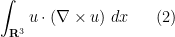
and (formally, at least) one has conservation of momentum

and angular momentum

(although, as we shall discuss below, due to the slow decay of at infinity, these integrals have to either be interpreted in a principal value sense, or else replaced with their vorticity-based formulations, namely impulse and moment of impulse). Total vorticity

is also conserved, although it turns out in three dimensions that this quantity vanishes when one assumes sufficient decay at infinity. Then there are the pointwise conservation laws: the vorticity and the volume form are both transported by the fluid flow, while the velocity field (when viewed as a covector) is transported up to a gradient; among other things, this gives the transport of vortex lines as well as Kelvin’s circulation theorem, and can also be used to deduce the helicity conservation law mentioned above. In my opinion, none of these laws actually prohibits a self-replicating computer from existing within the laws of ideal fluid flow, but they do significantly complicate the task of actually designing such a computer, or of the basic “gates” that such a computer would consist of.

Below the fold I would like to record and derive all the conservation laws mentioned above, which to my knowledge essentially form the complete set of known conserved quantities for the Euler equations. The material here (although not the notation) is drawn from this text of Majda and Bertozzi.

Polymath8b, IX: Large quadratic programs

This is the ninth thread for the Polymath8b project to obtain new bounds for the quantity

either for small values of (in particular ) or asymptotically as . The previous thread may be found here. The currently best known bounds on can be found at the wiki page.

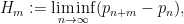
The focus is now on bounding unconditionally (in particular, without resorting to the Elliott-Halberstam conjecture or its generalisations). We can bound whenever one can find a symmetric square-integrable function supported on the simplex such that

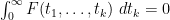
Our strategy for establishing this has been to restrict to be a linear combination of symmetrised monomials (restricted of course to ), where the degree is small; actually, it seems convenient to work with the slightly different basis where the are restricted to be even. The criterion (1) then becomes a large quadratic program with explicit but complicated rational coefficients. This approach has lowered down to , which led to the bound .

Actually, we know that the more general criterion

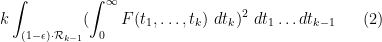
will suffice, whenever and is supported now on and obeys the vanishing marginal condition whenever . The latter is in particular obeyed when is supported on . A modification of the preceding strategy has lowered slightly to , giving the bound which is currently our best record.

However, the quadratic programs here have become extremely large and slow to run, and more efficient algorithms (or possibly more computer power) may be required to advance further.

Polymath8b, VIII: Time to start writing up the results?

This is the eighth thread for the Polymath8b project to obtain new bounds for the quantity

either for small values of (in particular ) or asymptotically as . The previous thread may be found here. The currently best known bounds on can be found at the wiki page.

The big news since the last thread is that we have managed to obtain the (sieve-theoretically) optimal bound of assuming the generalised Elliott-Halberstam conjecture (GEH), which pretty much closes off that part of the story. Unconditionally, our bound on is still . This bound was obtained using the “vanilla” Maynard sieve, in which the cutoff was supported in the original simplex , and only Bombieri-Vinogradov was used. In principle, we can enlarge the sieve support a little bit further now; for instance, we can enlarge to , but then have to shrink the J integrals to , provided that the marginals vanish for . However, we do not yet know how to numerically work with these expanded problems.

Given the substantial progress made so far, it looks like we are close to the point where we should declare victory and write up the results (though we should take one last look to see if there is any room to improve the bounds). There is actually a fair bit to write up:

• Improvements to the Maynard sieve (pushing beyond the simplex, the epsilon trick, and pushing beyond the cube);
• Asymptotic bounds for and hence ;
• Explicit bounds for (using the Polymath8a results)
• ;
• on GEH (and parity obstructions to any further improvement).

I will try to create a skeleton outline of such a paper in the Polymath8 Dropbox folder soon. It shouldn’t be nearly as big as the Polymath8a paper, but it will still be quite sizeable.

“New equidistribution estimates of Zhang type, and bounded gaps between primes” – and a retrospective

There are multiple purposes to this blog post.

The first purpose is to announce the uploading of the paper “New equidistribution estimates of Zhang type, and bounded gaps between primes” by D.H.J. Polymath, which is the main output of the Polymath8a project on bounded gaps between primes, to the arXiv, and to describe the main results of this paper below the fold.

The second purpose is to roll over the previous thread on all remaining Polymath8a-related matters (e.g. updates on the submission status of the paper) to a fresh thread. (Discussion of the ongoing Polymath8b project is however being kept on a separate thread, to try to reduce confusion.)

The final purpose of this post is to coordinate the writing of a retrospective article on the Polymath8 experience, which has been solicited for the Newsletter of the European Mathematical Society. I suppose that this could encompass both the Polymath8a and Polymath8b projects, even though the second one is still ongoing (but I think we will soon be entering the endgame there). I think there would be two main purposes of such a retrospective article. The first one would be to tell a story about the process of conducting mathematical research, rather than just describe the outcome of such research; this is an important aspect of the subject which is given almost no attention in most mathematical writing, and it would be good to be able to capture some sense of this process while memories are still relatively fresh. The other would be to draw some tentative conclusions with regards to what the strengths and weaknesses of a Polymath project are, and how appropriate such a format would be for other mathematical problems than bounded gaps between primes. In my opinion, the bounded gaps problem had some fairly unique features that made it particularly amenable to a Polymath project, such as (a) a high level of interest amongst the mathematical community in the problem; (b) a very focused objective (“improve !”), which naturally provided an obvious metric to measure progress; (c) the modular nature of the project, which allowed for people to focus on one aspect of the problem only, and still make contributions to the final goal; and (d) a very reasonable level of ambition (for instance, we did not attempt to prove the twin prime conjecture, which in my opinion would make a terrible Polymath project at our current level of mathematical technology). This is not an exhaustive list of helpful features of the problem; I would welcome other diagnoses of the project by other participants.

With these two objectives in mind, I propose a format for the retrospective article consisting of a brief introduction to the polymath concept in general and the polymath8 project in particular, followed by a collection of essentially independent contributions by different participants on their own experiences and thoughts. Finally we could have a conclusion section in which we make some general remarks on the polymath project (such as the remarks above). I’ve started a dropbox subfolder for this article (currently in a very skeletal outline form only), and will begin writing a section on my own experiences; other participants are of course encouraged to add their own sections (it is probably best to create separate files for these, and then input them into the main file retrospective.tex, to reduce edit conflicts. If there are participants who wish to contribute but do not currently have access to the Dropbox folder, please email me and I will try to have you added (or else you can supply your thoughts by email, or in the comments to this post; we may have a section for shorter miscellaneous comments from more casual participants, for people who don’t wish to write a lengthy essay on the subject).

As for deadlines, the EMS Newsletter would like a submitted article by mid-April in order to make the June issue, but in the worst case, it will just be held over until the issue after that.

Finite time blowup for an averaged three-dimensional Navier-Stokes equation

I’ve just uploaded to the arXiv the paper “Finite time blowup for an averaged three-dimensional Navier-Stokes equation“, submitted to J. Amer. Math. Soc.. The main purpose of this paper is to formalise the “supercriticality barrier” for the global regularity problem for the Navier-Stokes equation, which roughly speaking asserts that it is not possible to establish global regularity by any “abstract” approach which only uses upper bound function space estimates on the nonlinear part of the equation, combined with the energy identity. This is done by constructing a modification of the Navier-Stokes equations with a nonlinearity that obeys essentially all of the function space estimates that the true Navier-Stokes nonlinearity does, and which also obeys the energy identity, but for which one can construct solutions that blow up in finite time. Results of this type had been previously established by Montgomery-Smith, Gallagher-Paicu, and Li-Sinai for variants of the Navier-Stokes equation without the energy identity, and by Katz-Pavlovic and by Cheskidov for dyadic analogues of the Navier-Stokes equations in five and higher dimensions that obeyed the energy identity (see also the work of Plechac and Sverak and of Hou and Lei that also suggest blowup for other Navier-Stokes type models obeying the energy identity in five and higher dimensions), but to my knowledge this is the first blowup result for a Navier-Stokes type equation in three dimensions that also obeys the energy identity. Intriguingly, the method of proof in fact hints at a possible route to establishing blowup for the true Navier-Stokes equations, which I am now increasingly inclined to believe is the case (albeit for a very small set of initial data).

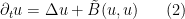
To state the results more precisely, recall that the Navier-Stokes equations can be written in the form

for a divergence-free velocity field and a pressure field , where is the viscosity, which we will normalise to be one. We will work in the non-periodic setting, so the spatial domain is , and for sake of exposition I will not discuss matters of regularity or decay of the solution (but we will always be working with strong notions of solution here rather than weak ones). Applying the Leray projection to divergence-free vector fields to this equation, we can eliminate the pressure, and obtain an evolution equation

purely for the velocity field, where is a certain bilinear operator on divergence-free vector fields (specifically, . The global regularity problem for Navier-Stokes is then equivalent to the global regularity problem for the evolution equation (1).

An important feature of the bilinear operator appearing in (1) is the cancellation law

(using the inner product on divergence-free vector fields), which leads in particular to the fundamental energy identity

This identity (and its consequences) provide essentially the only known a priori bound on solutions to the Navier-Stokes equations from large data and arbitrary times. Unfortunately, as discussed in this previous post, the quantities controlled by the energy identity are supercritical with respect to scaling, which is the fundamental obstacle that has defeated all attempts to solve the global regularity problem for Navier-Stokes without any additional assumptions on the data or solution (e.g. perturbative hypotheses, or a priori control on a critical norm such as the norm).

Our main result is then (slightly informally stated) as follows

Theorem 1 There exists an averaged version of the bilinear operator , of the form

for some probability space , some spatial rotation operators for , and some Fourier multipliers of order , for which one still has the cancellation law

and for which the averaged Navier-Stokes equation

admits solutions that blow up in finite time.

(There are some integrability conditions on the Fourier multipliers required in the above theorem in order for the conclusion to be non-trivial, but I am omitting them here for sake of exposition.)

Because spatial rotations and Fourier multipliers of order are bounded on most function spaces, automatically obeys almost all of the upper bound estimates that does. Thus, this theorem blocks any attempt to prove global regularity for the true Navier-Stokes equations which relies purely on the energy identity and on upper bound estimates for the nonlinearity; one must use some additional structure of the nonlinear operator which is not shared by an averaged version . Such additional structure certainly exists – for instance, the Navier-Stokes equation has a vorticity formulation involving only differential operators rather than pseudodifferential ones, whereas a general equation of the form (2) does not. However, “abstract” approaches to global regularity generally do not exploit such structure, and thus cannot be used to affirmatively answer the Navier-Stokes problem.

It turns out that the particular averaged bilinear operator that we will use will be a finite linear combination of local cascade operators, which take the form

where is a small parameter, are Schwartz vector fields whose Fourier transform is supported on an annulus, and is an -rescaled version of (basically a “wavelet” of wavelength about centred at the origin). Such operators were essentially introduced by Katz and Pavlovic as dyadic models for ; they have the essentially the same scaling property as (except that one can only scale along powers of , rather than over all positive reals), and in fact they can be expressed as an average of in the sense of the above theorem, as can be shown after a somewhat tedious amount of Fourier-analytic symbol manipulations.

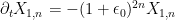
If we consider nonlinearities which are a finite linear combination of local cascade operators, then the equation (2) more or less collapses to a system of ODE in certain “wavelet coefficients” of . The precise ODE that shows up depends on what precise combination of local cascade operators one is using. Katz and Pavlovic essentially considered a single cascade operator together with its “adjoint” (needed to preserve the energy identity), and arrived (more or less) at the system of ODE

where are scalar fields for each integer . (Actually, Katz-Pavlovic worked with a technical variant of this particular equation, but the differences are not so important for this current discussion.) Note that the quadratic terms on the RHS carry a higher exponent of than the dissipation term; this reflects the supercritical nature of this evolution (the energy is monotone decreasing in this flow, so the natural size of given the control on the energy is ). There is a slight technical issue with the dissipation if one wishes to embed (3) into an equation of the form (2), but it is minor and I will not discuss it further here.

In principle, if the mode has size comparable to at some time , then energy should flow from to at a rate comparable to , so that by time or so, most of the energy of should have drained into the mode (with hardly any energy dissipated). Since the series is summable, this suggests finite time blowup for this ODE as the energy races ever more quickly to higher and higher modes. Such a scenario was indeed established by Katz and Pavlovic (and refined by Cheskidov) if the dissipation strength was weakened somewhat (the exponent has to be lowered to be less than ). As mentioned above, this is enough to give a version of Theorem 1 in five and higher dimensions.

On the other hand, it was shown a few years ago by Barbato, Morandin, and Romito that (3) in fact admits global smooth solutions (at least in the dyadic case , and assuming non-negative initial data). Roughly speaking, the problem is that as energy is being transferred from to , energy is also simultaneously being transferred from to , and as such the solution races off to higher modes a bit too prematurely, without absorbing all of the energy from lower modes. This weakens the strength of the blowup to the point where the moderately strong dissipation in (3) is enough to kill the high frequency cascade before a true singularity occurs. Because of this, the original Katz-Pavlovic model cannot quite be used to establish Theorem 1 in three dimensions. (Actually, the original Katz-Pavlovic model had some additional dispersive features which allowed for another proof of global smooth solutions, which is an unpublished result of Nazarov.)

To get around this, I had to “engineer” an ODE system with similar features to (3) (namely, a quadratic nonlinearity, a monotone total energy, and the indicated exponents of for both the dissipation term and the quadratic terms), but for which the cascade of energy from scale to scale was not interrupted by the cascade of energy from scale to scale . To do this, I needed to insert a delay in the cascade process (so that after energy was dumped into scale , it would take some time before the energy would start to transfer to scale ), but the process also needed to be abrupt (once the process of energy transfer started, it needed to conclude very quickly, before the delayed transfer for the next scale kicked in). It turned out that one could build a “quadratic circuit” out of some basic “quadratic gates” (analogous to how an electrical circuit could be built out of basic gates such as amplifiers or resistors) that achieved this task, leading to an ODE system essentially of the form

where is a suitable large parameter and is a suitable small parameter (much smaller than ). To visualise the dynamics of such a system, I found it useful to describe this system graphically by a “circuit diagram” that is analogous (but not identical) to the circuit diagrams arising in electrical engineering:

The coupling constants here range widely from being very large to very small; in practice, this makes the and modes absorb very little energy, but exert a sizeable influence on the remaining modes. If a lot of energy is suddenly dumped into , what happens next is roughly as follows: for a moderate period of time, nothing much happens other than a trickle of energy into , which in turn causes a rapid exponential growth of (from a very low base). After this delay, suddenly crosses a certain threshold, at which point it causes and to exchange energy back and forth with extreme speed. The energy from then rapidly drains into , and the process begins again (with a slight loss in energy due to the dissipation). If one plots the total energy as a function of time, it looks schematically like this:

As in the previous heuristic discussion, the time between cascades from one frequency scale to the next decay exponentially, leading to blowup at some finite time . (One could describe the dynamics here as being similar to the famous “lighting the beacons” scene in the Lord of the Rings movies, except that (a) as each beacon gets ignited, the previous one is extinguished, as per the energy identity; (b) the time between beacon lightings decrease exponentially; and (c) there is no soundtrack.)

There is a real (but remote) possibility that this sort of construction can be adapted to the true Navier-Stokes equations. The basic blowup mechanism in the averaged equation is that of a von Neumann machine, or more precisely a construct (built within the laws of the inviscid evolution ) that, after some time delay, manages to suddenly create a replica of itself at a finer scale (and to largely erase its original instantiation in the process). In principle, such a von Neumann machine could also be built out of the laws of the inviscid form of the Navier-Stokes equations (i.e. the Euler equations). In physical terms, one would have to build the machine purely out of an ideal fluid (i.e. an inviscid incompressible fluid). If one could somehow create enough “logic gates” out of ideal fluid, one could presumably build a sort of “fluid computer”, at which point the task of building a von Neumann machine appears to reduce to a software engineering exercise rather than a PDE problem (providing that the gates are suitably stable with respect to perturbations, but (as with actual computers) this can presumably be done by converting the analog signals of fluid mechanics into a more error-resistant digital form). The key thing missing in this program (in both senses of the word) to establish blowup for Navier-Stokes is to construct the logic gates within the laws of ideal fluids. (Compare with the situation for cellular automata such as Conway’s “Game of Life“, in which Turing complete computers, universal constructors, and replicators have all been built within the laws of that game.)