
You are currently browsing the monthly archive for March 2012.
I recently finished the first draft of the the first of my books, entitled “Hilbert’s fifth problem and related topics“, based on the lecture notes for my graduate course of the same name. The PDF of this draft is available here. As always, comments and corrections are welcome.
A few days ago, Endre Szemerédi was awarded the 2012 Abel prize “for his fundamental contributions to discrete mathematics and theoretical computer science, and in recognition of the profound and lasting impact of these contributions on additive number theory and ergodic theory.” The full citation for the prize may be found here, and the written notes for a talk given by Tim Gowers on Endre’s work at the announcement may be found here (and video of the talk can be found here).
As I was on the Abel prize committee this year, I won’t comment further on the prize, but will instead focus on what is arguably Endre’s most well known result, namely Szemerédi’s theorem on arithmetic progressions:
Theorem 1 (Szemerédi’s theorem) Let
be a set of integers of positive upper density, thus
, where
. Then
for any
.
Szemerédi’s original proof of this theorem is a remarkably intricate piece of combinatorial reasoning. Most proofs of theorems in mathematics – even long and difficult ones – generally come with a reasonably compact “high-level” overview, in which the proof is (conceptually, at least) broken down into simpler pieces. There may well be technical difficulties in formulating and then proving each of the component pieces, and then in fitting the pieces together, but usually the “big picture” is reasonably clear. To give just one example, the overall strategy of Perelman’s proof of the Poincaré conjecture can be briefly summarised as follows: to show that a simply connected three-dimensional manifold is homeomorphic to a sphere, place a Riemannian metric on it and perform Ricci flow, excising any singularities that arise by surgery, until the entire manifold becomes extinct. By reversing the flow and analysing the surgeries performed, obtain enough control on the topology of the original manifold to establish that it is a topological sphere.
In contrast, the pieces of Szemerédi’s proof are highly interlocking, particularly with regard to all the epsilon-type parameters involved; it takes quite a bit of notational setup and foundational lemmas before the key steps of the proof can even be stated, let alone proved. Szemerédi’s original paper contains a logical diagram of the proof (reproduced in Gowers’ recent talk) which already gives a fair indication of this interlocking structure. (Many years ago I tried to present the proof, but I was unable to find much of a simplification, and my exposition is probably not that much clearer than the original text.) Even the use of nonstandard analysis, which is often helpful in cleaning up armies of epsilons, turns out to be a bit tricky to apply here. (In typical applications of nonstandard analysis, one can get by with a single nonstandard universe, constructed as an ultrapower of the standard universe; but to correctly model all the epsilons occuring in Szemerédi’s argument, one needs to repeatedly perform the ultrapower construction to obtain a (finite) sequence of increasingly nonstandard (and increasingly saturated) universes, each one containing unbounded quantities that are far larger than any quantity that appears in the preceding universe, as discussed at the end of this previous blog post. This sequence of universes does end up concealing all the epsilons, but it is not so clear that this is a net gain in clarity for the proof; I may return to the nonstandard presentation of Szemeredi’s argument at some future juncture.)
Instead of trying to describe the entire argument here, I thought I would instead show some key components of it, with only the slightest hint as to how to assemble the components together to form the whole proof. In particular, I would like to show how two particular ingredients in the proof – namely van der Waerden’s theorem and the Szemerédi regularity lemma – become useful. For reasons that will hopefully become clearer later, it is convenient not only to work with ordinary progressions 

To illustrate some of the basic ideas, let us first consider a situation in which we have located a progression 


where 


If we write 


By hypothesis, we know already that each set 

Let us now make a “weakly mixing” assumption on the

for “most” subsets 


We will inductively consider the following (nonrigorously defined) sequence of claims 

-
, there are
arithmetic progressions
, such that
for all
.
(Actually, to avoid boundary issues one should restrict 


We can heuristically justify the claims 


which then gives the desired claim
The observant reader will note that we only needed the claim 

We now return to the question of how to justify the weak mixing hypothesis (2). For a single block
Proposition 2 (Single upper bound) Let
be a progression of progressions
. Suppose that for each
, the set
in
such that

Proof: The key is the double counting identity

Because

for each 

The claim then follows from the pigeonhole principle.

Now suppose we want to obtain weak mixing not just for a single set 

for all 


Proposition 3 (Multiple upper bound) Let
, let
. Then (if
simultaneously for all

Proof: Suppose that the claim failed (for some suitably large 
This can be viewed as a colouring of the interval 

One nice thing about this proposition is that the upper bounds can be automatically upgraded to an asymptotic:
Proposition 4 (Multiple mixing) Let
simultaneously for all
Proof: By applying the previous proposition to the collection of sets 

and

which gives the claim.
However, this improvement of Proposition 2 turns out to not be strong enough for applications. The reason is that the number 
Proposition 5 (Really multiple mixing) Let
in some (large) finite set
, let
be a subset of
. Then (if
simultaneously for almost all
.

Proof: We build a bipartite graph 


We now apply the regularity lemma to this graph 


and the number

The point here is that the 

simultaneously for all
This proposition now suggests a way forward to establish the type of mixing properties (2) needed for the preceding attempt at proving Szemerédi’s theorem to actually work. Whereas in that attempt, we were working with a single progression of progressions 


Of course, we still have to figure out how to get such large families of well-arranged progressions of progressions. Szemerédi’s solution was to begin by working with generalised progressions of a much larger rank 


This is an addendum to last quarter’s course notes on Hilbert’s fifth problem, which I am in the process of reviewing in order to transcribe them into a book (as was done similarly for several other sets of lecture notes on this blog). When reviewing the zeroth set of notes in particular, I found that I had made a claim (Proposition 11 from those notes) which asserted, roughly speaking, that any sufficiently large nilprogression was an approximate group, and promised to prove it later in the course when we had developed the ability to calculate efficiently in nilpotent groups. As it turned out, I managed finish the course without the need to develop these calculations, and so the proposition remained unproven. In order to rectify this, I will use this post to lay out some of the basic algebra of nilpotent groups, and use it to prove the above proposition, which turns out to be a bit tricky. (In my paper with Breuillard and Green, we avoid the need for this proposition by restricting attention to a special type of nilprogression, which we call a nilprogression in 
There are several ways to think about nilpotent groups; for instance one can use the model example of the Heisenberg group

over an arbitrary ring 

Another point of view, which arises naturally both in analysis and in algebraic geometry, is to view nilpotent groups as modeling “infinitesimal” perturbations of the identity, where the infinitesimals have a certain finite order. For instance, given a (not necessarily commutative) ring 


From a dynamical or group-theoretic perspective, one can also view nilpotent groups as towers of central extensions of a trivial group. Finitely generated nilpotent groups can also be profitably viewed as a special type of polycylic group; this is the perspective taken in this previous blog post. Last, but not least, one can view nilpotent groups from a combinatorial group theory perspective, as being words from some set of generators of various “degrees” subject to some commutation relations, with commutators of two low-degree generators being expressed in terms of higher degree objects, and all commutators of a sufficiently high degree vanishing. In particular, generators of a given degree can be moved freely around a word, as long as one is willing to generate commutator errors of higher degree.
With this last perspective, in particular, one can start computing in nilpotent groups by adopting the philosophy that the lowest order terms should be attended to first, without much initial concern for the higher order errors generated in the process of organising the lower order terms. Only after the lower order terms are in place should attention then turn to higher order terms, working successively up the hierarchy of degrees until all terms are dealt with. This turns out to be a relatively straightforward philosophy to implement in many cases (particularly if one is not interested in explicit expressions and constants, being content instead with qualitative expansions of controlled complexity), but the arguments are necessarily recursive in nature and as such can become a bit messy, and require a fair amount of notation to express precisely. So, unfortunately, the arguments here will be somewhat cumbersome and notation-heavy, even if the underlying methods of proof are relatively simple.
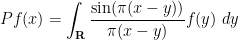
I’ve just uploaded to the arXiv my paper The asymptotic distribution of a single eigenvalue gap of a Wigner matrix, submitted to Probability Theory and Related Fields. This paper (like several of my previous papers) is concerned with the asymptotic distribution of the eigenvalues 


The location of an individual eigenvalue 

where the classical location ![{u = u_{i/n} \in [-2,2]}](https://s0.wp.com/latex.php?latex=%7Bu+%3D+u_%7Bi%2Fn%7D+%5Cin+%5B-2%2C2%5D%7D&bg=ffffff&fg=000000&s=0&c=20201002)
and the semicircular distribution 

Actually, one can improve the error term here from 


From the semicircle law (and the fundamental theorem of calculus), one expects the 


and ask what the distribution of 
As mentioned previously, we will focus on the bulk case 

![\displaystyle {\bf P}( N_{[\sqrt{n} u + \frac{x}{\sqrt{n} \rho_{sc}(u)}, \sqrt{n} u + \frac{y}{\sqrt{n} \rho_{sc}(u)}]} = 0) \ \ \ \ \ (1)](https://s0.wp.com/latex.php?latex=%5Cdisplaystyle+%7B%5Cbf+P%7D%28+N_%7B%5B%5Csqrt%7Bn%7D+u+%2B+%5Cfrac%7Bx%7D%7B%5Csqrt%7Bn%7D+%5Crho_%7Bsc%7D%28u%29%7D%2C+%5Csqrt%7Bn%7D+u+%2B+%5Cfrac%7By%7D%7B%5Csqrt%7Bn%7D+%5Crho_%7Bsc%7D%28u%29%7D%5D%7D+%3D+0%29+%5C+%5C+%5C+%5C+%5C+%281%29&bg=ffffff&fg=000000&s=0&c=20201002)
that an interval ![{[\sqrt{n} u + \frac{x}{\sqrt{n} \rho_{sc}(u)}, \sqrt{n} u + \frac{y}{\sqrt{n} \rho_{sc}(u)}]}](https://s0.wp.com/latex.php?latex=%7B%5B%5Csqrt%7Bn%7D+u+%2B+%5Cfrac%7Bx%7D%7B%5Csqrt%7Bn%7D+%5Crho_%7Bsc%7D%28u%29%7D%2C+%5Csqrt%7Bn%7D+u+%2B+%5Cfrac%7By%7D%7B%5Csqrt%7Bn%7D+%5Crho_%7Bsc%7D%28u%29%7D%5D%7D&bg=ffffff&fg=000000&s=0&c=20201002)


![\displaystyle \det( 1 - 1_{[x,y]} P 1_{[x,y]} ) + o(1),](https://s0.wp.com/latex.php?latex=%5Cdisplaystyle+%5Cdet%28+1+-+1_%7B%5Bx%2Cy%5D%7D+P+1_%7B%5Bx%2Cy%5D%7D+%29+%2B+o%281%29%2C&bg=ffffff&fg=000000&s=0&c=20201002)
where
to Fourier modes in ![{[-1/2,1/2]}](https://s0.wp.com/latex.php?latex=%7B%5B-1%2F2%2C1%2F2%5D%7D&bg=ffffff&fg=000000&s=0&c=20201002)


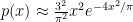
![\displaystyle p(x) := \frac{d^2}{dx^2} \det( 1 - 1_{[0,x]} P 1_{[0,x]} ).](https://s0.wp.com/latex.php?latex=%5Cdisplaystyle+p%28x%29+%3A%3D+%5Cfrac%7Bd%5E2%7D%7Bdx%5E2%7D+%5Cdet%28+1+-+1_%7B%5B0%2Cx%5D%7D+P+1_%7B%5B0%2Cx%5D%7D+%29.&bg=ffffff&fg=000000&s=0&c=20201002)
A reasonably accurate approximation for 


Unfortunately, when one tries to make this argument rigorous, one finds that the asymptotic for (1) does not control a single gap ![{[i_0 - L, i_0 + L]}](https://s0.wp.com/latex.php?latex=%7B%5Bi_0+-+L%2C+i_0+%2B+L%5D%7D&bg=ffffff&fg=000000&s=0&c=20201002)


The problem is that when one specifies a given window of spectrum such as 
The main difficulty here is that there could potentially be some strange coupling between the event (1) of an interval being devoid of eigenvalues, and the number 
The main result of the current paper is that these anomalies do not actually occur, and that all of the eigenvalue gaps
The main task in the proof is to show that the random variable ![{1 - 1_{[x,y]}P1_{[x,y]}}](https://s0.wp.com/latex.php?latex=%7B1+-+1_%7B%5Bx%2Cy%5D%7DP1_%7B%5Bx%2Cy%5D%7D%7D&bg=ffffff&fg=000000&s=0&c=20201002)
![{[x,y]}](https://s0.wp.com/latex.php?latex=%7B%5Bx%2Cy%5D%7D&bg=ffffff&fg=000000&s=0&c=20201002)
In this final set of course notes, we discuss how (a generalisation of) the expansion results obtained in the preceding notes can be used for some number-theoretic applications, and in particular to locate almost primes inside orbits of thin groups, following the work of Bourgain, Gamburd, and Sarnak. We will not attempt here to obtain the sharpest or most general results in this direction, but instead focus on the simplest instances of these results which are still illustrative of the ideas involved.
One of the basic general problems in analytic number theory is to locate tuples of primes of a certain form; for instance, the famous (and still unsolved) twin prime conjecture asserts that there are infinitely many pairs 


More generally, given some explicit subset 


At this level of generality, this problem is impossibly difficult. Indeed, even the much simpler problem of deciding whether the set 


Even in this simpler setting, the question of determining whether an orbit 


On the other hand, much more is known if one is willing to replace the primes by the larger set of almost primes – integers with a small number of prime factors (counting multiplicity). Specifically, for any 


The main tool that allows one to count almost primes in orbits is sieve theory. The reason for this lies in the simple observation that in order to ensure that an integer 

The most basic sieve of this form is the sieve of Eratosthenes, which when combined with the inclusion-exclusion principle gives the Legendre sieve (or exact sieve), which gives an exact formula for quantities such as the number 


Very roughly speaking, the end result of sieve theory is that excepting some degenerate and “exponentially thin” settings (such as those associated with the Mersenne primes), all the orbits which are expected to have a large number of primes, can be proven to at least have a large number of
Theorem 1 (Bourgain-Gamburd-Sarnak) Let
which is not virtually solvable. Let
be a polynomial with integer coefficients obeying the following primitivity condition: for any positive integer
, there exists
such that
is coprime to
with
This is not the strongest version of the Bourgain-Gamburd-Sarnak theorem, but it captures the general flavour of their results. Note that the theorem immediately implies an analogous result for orbits 


By specialising to the polynomial 
It turns out that to prove Theorem 1, the Cayley expansion results in 


Recent Comments