You are currently browsing the monthly archive for June 2011.

Following the results from the recent poll on this blog, the mini-polymath3 project (which will focus on one of the problems from the 2011 IMO) will start at July 19 8pm UTC, and be run concurrently on this blog, on the polymath wiki, and on the polymath blog.

Over the past few months or so, I have been brushing up on my Lie group theory, as part of my project to fully understand the theory surrounding Hilbert’s fifth problem. Every so often, I encounter a basic fact in Lie theory which requires a slightly non-trivial “trick” to prove; I am recording two of them here, so that I can find these tricks again when I need to.

The first fact concerns the exponential map {\exp: {\mathfrak g} \rightarrow G} from a Lie algebra {{\mathfrak g}} of a Lie group {G} to that group. (For this discussion we will only consider finite-dimensional Lie groups and Lie algebras over the reals {{\bf R}}.) A basic fact in the subject is that the exponential map is locally a homeomorphism: there is a neighbourhood of the origin in {{\mathfrak g}} that is mapped homeomorphically by the exponential map to a neighbourhood of the identity in {G}. This local homeomorphism property is the foundation of an important dictionary between Lie groups and Lie algebras.

It is natural to ask whether the exponential map is globally a homeomorphism, and not just locally: in particular, whether the exponential map remains both injective and surjective. For instance, this is the case for connected, simply connected, nilpotent Lie groups (as can be seen from the Baker-Campbell-Hausdorff formula.)

The circle group {S^1}, which has {{\bf R}} as its Lie algebra, already shows that global injectivity fails for any group that contains a circle subgroup, which is a huge class of examples (including, for instance, the positive dimensional compact Lie groups, or non-simply-connected Lie groups). Surjectivity also obviously fails for disconnected groups, since the Lie algebra is necessarily connected, and so the image under the exponential map must be connected also. However, even for connected Lie groups, surjectivity can fail. To see this, first observe that if the exponential map was surjective, then every group element {g \in G} has a square root (i.e. an element {h \in G} with {h^2 = g}), since {\exp(x)} has {\exp(x/2)} as a square root for any {x \in {\mathfrak g}}. However, there exist elements in connected Lie groups without square roots. A simple example is provided by the matrix

\displaystyle  g = \begin{pmatrix} -4 & 0 \\ 0 & -1/4 \end{pmatrix}

in the connected Lie group {SL_2({\bf R})}. This matrix has eigenvalues {-4}, {-1/4}. Thus, if {h \in SL_2({\bf R})} is a square root of {g}, we see (from the Jordan normal form) that it must have at least one eigenvalue in {\{-2i,+2i\}}, and at least one eigenvalue in {\{-i/2,i/2\}}. On the other hand, as {h} has real coefficients, the complex eigenvalues must come in conjugate pairs {\{ a+bi, a-bi\}}. Since {h} can only have at most {2} eigenvalues, we obtain a contradiction.

However, there is an important case where surjectivity is recovered:

Proposition 1 If {G} is a compact connected Lie group, then the exponential map is surjective.

Proof: The idea here is to relate the exponential map in Lie theory to the exponential map in Riemannian geometry. We first observe that every compact Lie group {G} can be given the structure of a Riemannian manifold with a bi-invariant metric. This can be seen in one of two ways. Firstly, one can put an arbitrary positive definite inner product on {{\mathfrak g}} and average it against the adjoint action of {G} using Haar probability measure (which is available since {G} is compact); this gives an ad-invariant positive-definite inner product on {{\mathfrak g}} that one can then translate by either left or right translation to give a bi-invariant Riemannian structure on {G}. Alternatively, one can use the Peter-Weyl theorem to embed {G} in a unitary group {U(n)}, at which point one can induce a bi-invariant metric on {G} from the one on the space {M_n({\bf C}) \equiv {\bf C}^{n^2}} of {n \times n} complex matrices.

As {G} is connected and compact and thus complete, we can apply the Hopf-Rinow theorem and conclude that any two points are connected by at least one geodesic, so that the Riemannian exponential map from {{\mathfrak g}} to {G} formed by following geodesics from the origin is surjective. But one can check that the Lie exponential map and Riemannian exponential map agree; for instance, this can be seen by noting that the group structure naturally defines a connection on the tangent bundle which is both torsion-free and preserves the bi-invariant metric, and must therefore agree with the Levi-Civita metric. (Alternatively, one can embed into a unitary group {U(n)} and observe that {G} is totally geodesic inside {U(n)}, because the geodesics in {U(n)} can be described explicitly in terms of one-parameter subgroups.) The claim follows. \Box

Remark 1 While it is quite nice to see Riemannian geometry come in to prove this proposition, I am curious to know if there is any other proof of surjectivity for compact connected Lie groups that does not require explicit introduction of Riemannian geometry concepts.

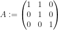
The other basic fact I learned recently concerns the algebraic nature of Lie groups and Lie algebras. An important family of examples of Lie groups are the algebraic groups – algebraic varieties with a group law given by algebraic maps. Given that one can always automatically upgrade the smooth structure on a Lie group to analytic structure (by using the Baker-Campbell-Hausdorff formula), it is natural to ask whether one can upgrade the structure further to an algebraic structure. Unfortunately, this is not always the case. A prototypical example of this is given by the one-parameter subgroup
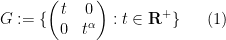
\displaystyle  G := \{ \begin{pmatrix} t & 0 \\ 0 & t^\alpha \end{pmatrix}: t \in {\bf R}^+ \} \ \ \ \ \ (1)

of {GL_2({\bf R})}. This is a Lie group for any exponent {\alpha \in {\bf R}}, but if {\alpha} is irrational, then the curve that {G} traces out is not an algebraic subset of {GL_2({\bf R})} (as one can see by playing around with Puiseux series).

This is not a true counterexample to the claim that every Lie group can be given the structure of an algebraic group, because one can give {G} a different algebraic structure than one inherited from the ambient group {GL_2({\bf R})}. Indeed, {G} is clearly isomorphic to the additive group {{\bf R}}, which is of course an algebraic group. However, a modification of the above construction works:

Proposition 2 There exists a Lie group {G} that cannot be given the structure of an algebraic group.

Proof: We use an example from the text of Tauvel and Yu (that I found via this MathOverflow posting). We consider the subgroup
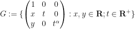
\displaystyle  G := \{ \begin{pmatrix} 1 & 0 & 0 \\ x & t & 0 \\ y & 0 & t^\alpha \end{pmatrix}: x, y \in {\bf R}; t \in {\bf R}^+ \}

of {GL_3({\bf R})}, with {\alpha} an irrational number. This is a three-dimensional (metabelian) Lie group, whose Lie algebra {{\mathfrak g} \subset {\mathfrak gl}_3({\bf R})} is spanned by the elements

\displaystyle  X := \begin{pmatrix} 0 & 0 & 0 \\ 0 & 1 & 0 \\ 0 & 0 & \alpha \end{pmatrix}

\displaystyle  Y := \begin{pmatrix} 0 & 0 & 0 \\ -1 & 0 & 0 \\ 0 & 0 & 0 \end{pmatrix}

\displaystyle  Z := \begin{pmatrix} 0 & 0 & 0 \\ 0 & 0 & 0 \\ -\alpha & 0 & 0 \end{pmatrix}

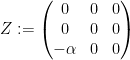
with the Lie bracket given by

\displaystyle  [Y,X] = -Y; [Z,X] = -\alpha Z; [Y,Z] = 0.

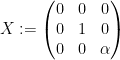
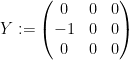
As such, we see that if we use the basis {X, Y, Z} to identify {{\mathfrak g}} to {{\bf R}^3}, then adjoint representation of {G} is the identity map.

If {G} is an algebraic group, it is easy to see that the adjoint representation {\hbox{Ad}: G \rightarrow GL({\mathfrak g})} is also algebraic, and so {\hbox{Ad}(G) = G} is algebraic in {GL({\mathfrak g})}. Specialising to our specific example, in which adjoint representation is the identity, we conclude that if {G} has any algebraic structure, then it must also be an algebraic subgroup of {GL_3({\bf R})}; but {G} projects to the group (1) which is not algebraic, a contradiction. \Box

A slight modification of the same argument also shows that not every Lie algebra is algebraic, in the sense that it is isomorphic to a Lie algebra of an algebraic group. (However, there are important classes of Lie algebras that are automatically algebraic, such as nilpotent or semisimple Lie algebras.)

Let {G} be a Lie group with Lie algebra {{\mathfrak g}}. As is well known, the exponential map {\exp: {\mathfrak g} \rightarrow G} is a local homeomorphism near the identity. As such, the group law on {G} can be locally pulled back to an operation {*: U \times U \rightarrow {\mathfrak g}} defined on a neighbourhood {U} of the identity in {G}, defined as

\displaystyle  x * y := \log( \exp(x) \exp(y) )

where {\log} is the local inverse of the exponential map. One can view {*} as the group law expressed in local exponential coordinates around the origin.

An asymptotic expansion for {x*y} is provided by the Baker-Campbell-Hausdorff (BCH) formula

\displaystyle  x*y = x+y+ \frac{1}{2} [x,y] + \frac{1}{12}[x,[x,y]] - \frac{1}{12}[y,[x,y]] + \ldots

for all sufficiently small {x,y}, where {[,]: {\mathfrak g} \times {\mathfrak g} \rightarrow {\mathfrak g}} is the Lie bracket. More explicitly, one has the Baker-Campbell-Hausdorff-Dynkin formula

\displaystyle  x * y = x + \int_0^1 F( \hbox{Ad}_x \hbox{Ad}_{ty} ) y\ dt \ \ \ \ \ (1)

for all sufficiently small {x,y}, where {\hbox{Ad}_x = \exp( \hbox{ad}_x )}, {\hbox{ad}_x: {\bf R}^d \rightarrow {\bf R}^d} is the adjoint representation {\hbox{ad}_x(y) := [x,y]}, and {F} is the function

\displaystyle  F( t ) := \frac{t \log t}{t-1}

which is real analytic near {t=1} and can thus be applied to linear operators sufficiently close to the identity. One corollary of this is that the multiplication operation {*} is real analytic in local coordinates, and so every smooth Lie group is in fact a real analytic Lie group.

It turns out that one does not need the full force of the smoothness hypothesis to obtain these conclusions. It is, for instance, a classical result that {C^2} regularity of the group operations is already enough to obtain the Baker-Campbell-Hausdorff formula. Actually, it turns out that we can weaken this a bit, and show that even {C^{1,1}} regularity (i.e. that the group operations are continuously differentiable, and the derivatives are locally Lipschitz) is enough to make the classical derivation of the Baker-Campbell-Hausdorff formula work. More precisely, we have

Theorem 1 ({C^{1,1}} Baker-Campbell-Hausdorff formula) Let {{\bf R}^d} be a finite-dimensional vector space, and suppose one has a continuous operation {*: U \times U \rightarrow {\bf R}^d} defined on a neighbourhood {U} around the origin, which obeys the following three axioms:

  • (Approximate additivity) For {x,y} sufficiently close to the origin, one has

    \displaystyle  x*y = x+y+O(|x| |y|). \ \ \ \ \ (2)

    (In particular, {0*x=x*0=x} for {x} sufficiently close to the origin.)

  • (Associativity) For {x,y,z} sufficiently close to the origin, {(x*y)*z = x*(y*z)}.
  • (Radial homogeneity) For {x} sufficiently close to the origin, one has

    \displaystyle  (sx) * (tx) = (s+t)x \ \ \ \ \ (3)

    for all {s,t \in [-1,1]}. (In particular, {x * (-x) = (-x) * x = 0} for all {x} sufficiently close to the origin.)

Then {*} is real analytic (and in particular, smooth) near the origin. (In particular, {*} gives a neighbourhood of the origin the structure of a local Lie group.)

Indeed, we will recover the Baker-Campbell-Hausdorff-Dynkin formula (after defining {\hbox{Ad}_x} appropriately) in this setting; see below the fold.

The reason that we call this a {C^{1,1}} Baker-Campbell-Hausdorff formula is that if the group operation {*} has {C^{1,1}} regularity, and has {0} as an identity element, then Taylor expansion already gives (2), and in exponential coordinates (which, as it turns out, can be defined without much difficulty in the {C^{1,1}} category) one automatically has (3).

We will record the proof of Theorem 1 below the fold; it largely follows the classical derivation of the BCH formula, but due to the low regularity one will rely on tools such as telescoping series and Riemann sums rather than on the fundamental theorem of calculus. As an application of this theorem, we can give an alternate derivation of one of the components of the solution to Hilbert’s fifth problem, namely the construction of a Lie group structure from a Gleason metric, which was covered in the previous post; we discuss this at the end of this article. With this approach, one can avoid any appeal to von Neumann’s theorem and Cartan’s theorem (discussed in this post), or the Kuranishi-Gleason extension theorem (discussed in this post).

Read the rest of this entry »

Hilbert’s fifth problem asks to clarify the extent that the assumption on a differentiable or smooth structure is actually needed in the theory of Lie groups and their actions. While this question is not precisely formulated and is thus open to some interpretation, the following result of Gleason and Montgomery-Zippin answers at least one aspect of this question:

Theorem 1 (Hilbert’s fifth problem) Let {G} be a topological group which is locally Euclidean (i.e. it is a topological manifold). Then {G} is isomorphic to a Lie group.

Theorem 1 can be viewed as an application of the more general structural theory of locally compact groups. In particular, Theorem 1 can be deduced from the following structural theorem of Gleason and Yamabe:

Theorem 2 (Gleason-Yamabe theorem) Let {G} be a locally compact group, and let {U} be an open neighbourhood of the identity in {G}. Then there exists an open subgroup {G'} of {G}, and a compact subgroup {N} of {G'} contained in {U}, such that {G'/N} is isomorphic to a Lie group.

The deduction of Theorem 1 from Theorem 2 proceeds using the Brouwer invariance of domain theorem and is discussed in this previous post. In this post, I would like to discuss the proof of Theorem 2. We can split this proof into three parts, by introducing two additional concepts. The first is the property of having no small subgroups:

Definition 3 (NSS) A topological group {G} is said to have no small subgroups, or is NSS for short, if there is an open neighbourhood {U} of the identity in {G} that contains no subgroups of {G} other than the trivial subgroup {\{ \hbox{id}\}}.

An equivalent definition of an NSS group is one which has an open neighbourhood {U} of the identity that every non-identity element {g \in G \backslash \{\hbox{id}\}} escapes in finite time, in the sense that {g^n \not \in U} for some positive integer {n}. It is easy to see that all Lie groups are NSS; we shall shortly see that the converse statement (in the locally compact case) is also true, though significantly harder to prove.

Another useful property is that of having what I will call a Gleason metric:

Definition 4 Let {G} be a topological group. A Gleason metric on {G} is a left-invariant metric {d: G \times G \rightarrow {\bf R}^+} which generates the topology on {G} and obeys the following properties for some constant {C>0}, writing {\|g\|} for {d(g,\hbox{id})}:

  • (Escape property) If {g \in G} and {n \geq 1} is such that {n \|g\| \leq \frac{1}{C}}, then {\|g^n\| \geq \frac{1}{C} n \|g\|}.
  • (Commutator estimate) If {g, h \in G} are such that {\|g\|, \|h\| \leq \frac{1}{C}}, then

    \displaystyle  \|[g,h]\| \leq C \|g\| \|h\|, \ \ \ \ \ (1)

    where {[g,h] := g^{-1}h^{-1}gh} is the commutator of {g} and {h}.

For instance, the unitary group {U(n)} with the operator norm metric {d(g,h) := \|g-h\|_{op}} can easily verified to be a Gleason metric, with the commutator estimate (1) coming from the inequality

\displaystyle  \| [g,h] - 1 \|_{op} = \| gh - hg \|_{op}

\displaystyle  = \| (g-1) (h-1) - (h-1) (g-1) \|_{op}

\displaystyle  \leq 2 \|g-1\|_{op} \|g-1\|_{op}.

Similarly, any left-invariant Riemannian metric on a (connected) Lie group can be verified to be a Gleason metric. From the escape property one easily sees that all groups with Gleason metrics are NSS; again, we shall see that there is a partial converse.

Remark 1 The escape and commutator properties are meant to capture “Euclidean-like” structure of the group. Other metrics, such as Carnot-Carathéodory metrics on Carnot Lie groups such as the Heisenberg group, usually fail one or both of these properties.

The proof of Theorem 2 can then be split into three subtheorems:

Theorem 5 (Reduction to the NSS case) Let {G} be a locally compact group, and let {U} be an open neighbourhood of the identity in {G}. Then there exists an open subgroup {G'} of {G}, and a compact subgroup {N} of {G'} contained in {U}, such that {G'/N} is NSS, locally compact, and metrisable.

Theorem 6 (Gleason’s lemma) Let {G} be a locally compact metrisable NSS group. Then {G} has a Gleason metric.

Theorem 7 (Building a Lie structure) Let {G} be a locally compact group with a Gleason metric. Then {G} is isomorphic to a Lie group.

Clearly, by combining Theorem 5, Theorem 6, and Theorem 7 one obtains Theorem 2 (and hence Theorem 1).

Theorem 5 and Theorem 6 proceed by some elementary combinatorial analysis, together with the use of Haar measure (to build convolutions, and thence to build “smooth” bump functions with which to create a metric, in a variant of the analysis used to prove the Birkhoff-Kakutani theorem); Theorem 5 also requires Peter-Weyl theorem (to dispose of certain compact subgroups that arise en route to the reduction to the NSS case), which was discussed previously on this blog.

In this post I would like to detail the final component to the proof of Theorem 2, namely Theorem 7. (I plan to discuss the other two steps, Theorem 5 and Theorem 6, in a separate post.) The strategy is similar to that used to prove von Neumann’s theorem, as discussed in this previous post (and von Neumann’s theorem is also used in the proof), but with the Gleason metric serving as a substitute for the faithful linear representation. Namely, one first gives the space {L(G)} of one-parameter subgroups of {G} enough of a structure that it can serve as a proxy for the “Lie algebra” of {G}; specifically, it needs to be a vector space, and the “exponential map” needs to cover an open neighbourhood of the identity. This is enough to set up an “adjoint” representation of {G}, whose image is a Lie group by von Neumann’s theorem; the kernel is essentially the centre of {G}, which is abelian and can also be shown to be a Lie group by a similar analysis. To finish the job one needs to use arguments of Kuranishi and of Gleason, as discussed in this previous post.

The arguments here can be phrased either in the standard analysis setting (using sequences, and passing to subsequences often) or in the nonstandard analysis setting (selecting an ultrafilter, and then working with infinitesimals). In my view, the two approaches have roughly the same level of complexity in this case, and I have elected for the standard analysis approach.

Remark 2 From Theorem 7 we see that a Gleason metric structure is a good enough substitute for smooth structure that it can actually be used to reconstruct the entire smooth structure; roughly speaking, the commutator estimate (1) allows for enough “Taylor expansion” of expressions such as {g^n h^n} that one can simulate the fundamentals of Lie theory (in particular, construction of the Lie algebra and the exponential map, and its basic properties. The advantage of working with a Gleason metric rather than a smoother structure, though, is that it is relatively undemanding with regards to regularity; in particular, the commutator estimate (1) is roughly comparable to the imposition {C^{1,1}} structure on the group {G}, as this is the minimal regularity to get the type of Taylor approximation (with quadratic errors) that would be needed to obtain a bound of the form (1). We will return to this point in a later post.

Read the rest of this entry »

We recall Brouwer’s famous fixed point theorem:

Theorem 1 (Brouwer fixed point theorem) Let {f: B^n \rightarrow B^n} be a continuous function on the unit ball {B^n := \{ x \in {\bf R}^n: \|x\| \leq 1 \}} in a Euclidean space {{\bf R}^n}. Then {f} has at least one fixed point, thus there exists {x \in B^n} with {f(x)=x}.

This theorem has many proofs, most of which revolve (either explicitly or implicitly) around the notion of the degree of a continuous map {f: S^{n-1} \rightarrow S^{n-1}} of the unit sphere {S^{n-1} := \{ x \in {\bf R}^n: \|x\|=1\}} to itself, and more precisely around the stability of degree with respect to homotopy. (Indeed, one can view the Brouwer fixed point theorem as an assertion that some non-trivial degree-like invariant must exist, or more abstractly that the homotopy group {\pi_{n-1}(S^{n-1})} is non-trivial.)

One of the many applications of this result is to prove Brouwer’s invariance of domain theorem:

Theorem 2 (Brouwer invariance of domain theorem) Let {U} be an open subset of {{\bf R}^n}, and let {f: U \rightarrow {\bf R}^n} be a continuous injective map. Then {f(U)} is also open.

This theorem in turn has an important corollary:

Corollary 3 (Topological invariance of dimension) If {n > m}, and {U} is a non-empty open subset of {{\bf R}^n}, then there is no continuous injective mapping from {U} to {{\bf R}^m}. In particular, {{\bf R}^n} and {{\bf R}^m} are not homeomorphic.

This corollary is intuitively obvious, but note that topological intuition is not always rigorous. For instance, it is intuitively plausible that there should be no continuous surjection from {{\bf R}^m} to {{\bf R}^n} for {n>m}, but such surjections always exist, thanks to variants of the Peano curve construction.

Theorem 2 or Corollary 3 can be proven by simple ad hoc means for small values of {n} or {m} (for instance, by noting that removing a point from {{\bf R}^n} will disconnect {{\bf R}^n} when {n=1}, but not for {n>1}), but I do not know of any proof of these results in general dimension that does not require algebraic topology machinery that is at least as sophisticated as the Brouwer fixed point theorem. (Lebesgue, for instance, famously failed to establish the above corollary rigorously, although he did end up discovering the important concept of Lebesgue covering dimension as a result of his efforts.)

Nowadays, the invariance of domain theorem is usually proven using the machinery of singular homology. In this post I would like to record a short proof of Theorem 2 using Theorem 1 that I discovered in a paper of Kulpa, which avoids any use of algebraic topology tools beyond the fixed point theorem, though it is more ad hoc in its approach than the systematic singular homology approach.

Remark 1 A heuristic explanation as to why the Brouwer fixed point theorem is more or less a necessary ingredient in the proof of the invariance of domain theorem is that a counterexample to the former result could conceivably be used to create a counterexample to the latter one. Indeed, if the Brouwer fixed point theorem failed, then (as is well known) one would be able to find a continuous function {F: B^n \rightarrow S^{n-1}} that was the identity on {S^{n-1}} (indeed, one could take {F(x)} to be the first point in which the ray from {f(x)} through {x} hits {S^{n-1}}). If one then considered the function {G: B^n \rightarrow {\bf R}^n} defined by {G(x) := (1+\|x\|) F(x)}, then this would be a continuous function which avoids the interior of {B^n}, but which maps the origin {0} to a point on the sphere {S^{n-1}} (and maps {S^{n-1}} to the dilate {2 \cdot S^{n-1}}). This could conceivably be a counterexample to Theorem 2, except that {G} is not necessarily injective. I do not know if there is a more rigorous way to formulate this connection.

The reason I was looking for a proof of the invariance of domain theorem was that it comes up in the very last stage of the solution to Hilbert’s fifth problem, namely to establish the following fact:

Theorem 4 (Hilbert’s fifth problem) Every locally Euclidean group is isomorphic to a Lie group.

Recall that a locally Euclidean group is a topological group which is locally homeomorphic to an open subset of a Euclidean space {{\bf R}^n}, i.e. it is a continuous manifold. Note in contrast that a Lie group is a topological group which is locally diffeomorphic to an open subset of {{\bf R}^n}, it is a smooth manifold. Thus, Hilbert’s fifth problem is a manifestation of the “rigidity” of algebraic structure (in this case, group structure), which turns weak regularity (continuity) into strong regularity (smoothness).

It is plausible that something like Corollary 3 would need to be invoked in order to solve Hilbert’s fifth problem. After all, if Euclidean spaces {{\bf R}^n}, {{\bf R}^m} of different dimension were homeomorphic to each other, then the property of being locally Euclidean loses a lot of meaning, and would thus not be a particularly powerful hypothesis. Note also that it is clear that two Lie groups can only be isomorphic if they have the same dimension, so in view of Theorem 4, it becomes plausible that two Euclidean spaces can only be homeomorphic if they have the same dimension, although I do not know of a way to rigorously deduce this claim from Theorem 4.

Interestingly, Corollary 3 is the only place where algebraic topology enters into the solution of Hilbert’s fifth problem (although its cousin, point-set topology, is used all over the place). There are results closely related to Theorem 4, such as the Gleason-Yamabe theorem mentioned in a recent post, which do not use the notion of being locally Euclidean, and do not require algebraic topological methods in their proof. Indeed, one can deduce Theorem 4 from the Gleason-Yamabe theorem and invariance of domain; we sketch a proof of this (following Montgomery and Zippin) below the fold.

Read the rest of this entry »

In the last two years, I ran a “mini-polymath” project to solve one of the problems of that year’s International Mathematical Olympiad (IMO).  This year, the IMO is being held in the Netherlands, with the problems being released on July 18 and 19, and I am planning to once again select a question (most likely the last question Q6, but I’ll exercise my discretion on which problem to select once I see all of them).

The format of the last year’s mini-polymath project seemed to work well, so I am inclined to simply repeat that format without much modification this time around, in order to collect a consistent set of data about these projects.  Thus, unles the plan changes, the project will start at a pre-arranged time and date, with plenty of advance notice, and be run simultaneously on three different sites: a “research thread” over at the polymath blog for the problem solving process, a “discussion thread” over at this blog for any meta-discussion about the project, and a wiki page at the polymath wiki to record the progress already made at the research thread.  (Incidentally, there is a current discussion at the wiki about the logo for that site; please feel free to chip in your opinion on the various proposed icons.)  The project will follow the usual polymath rules (as summarised for instance in the 2010 mini-polymath thread).

There are some kinks with our format that still need to be worked out, unfortunately; the two main ones that keep recurring in previous feedback are (a) there is no way to edit or preview comments without the intervention of one of the blog maintainers, and (b) even with comment threading, it is difficult to keep track of all the multiple discussions going on at once.  It is conceivable that we could use a different forum than the WordPress-based blogs we have been using for previous projects for this mini-polymath to experiment with other software that may help ameliorate (a) and (b) (though any alternative site should definitely have the ability to support some sort of TeX, and should be easily accessible by polymath participants, without the need for a cumbersome registration process); if there are any suggestions for such alternatives, I would be happy to hear about them in the comments to this post.  (Of course, any other comments germane to the polymath or mini-polymath projects would also be appropriate for the comment thread.)

The other thing to do at this early stage is set up a poll for the start time for the project (and also to gauge interest in participation).  For ease of comparison I am going to use the same four-hour time slots as for the 2010 poll.  All times are in Coordinated Universal Time (UTC), which is essentially the same as GMT; conversions between UTC and local time zones can for instance be found on this web site.   For instance, the Netherlands are at UTC+2, and so July 19 4m UTC (say) would be July 19 6pm in Netherlands local time.  (I myself will be at UTC-7.)

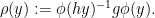
In the last few months, I have been working my way through the theory behind the solution to Hilbert’s fifth problem, as I (together with Emmanuel Breuillard, Ben Green, and Tom Sanders) have found this theory to be useful in obtaining noncommutative inverse sumset theorems in arbitrary groups; I hope to be able to report on this connection at some later point on this blog. Among other things, this theory achieves the remarkable feat of creating a smooth Lie group structure out of what is ostensibly a much weaker structure, namely the structure of a locally compact group. The ability of algebraic structure (in this case, group structure) to upgrade weak regularity (in this case, continuous structure) to strong regularity (in this case, smooth and even analytic structure) seems to be a recurring theme in mathematics, and an important part of what I like to call the “dichotomy between structure and randomness”.

The theory of Hilbert’s fifth problem sprawls across many subfields of mathematics: Lie theory, representation theory, group theory, nonabelian Fourier analysis, point-set topology, and even a little bit of group cohomology. The latter aspect of this theory is what I want to focus on today. The general question that comes into play here is the extension problem: given two (topological or Lie) groups {H} and {K}, what is the structure of the possible groups {G} that are formed by extending {H} by {K}. In other words, given a short exact sequence

\displaystyle  0 \rightarrow K \rightarrow G \rightarrow H \rightarrow 0,

to what extent is the structure of {G} determined by that of {H} and {K}?

As an example of why understanding the extension problem would help in structural theory, let us consider the task of classifying the structure of a Lie group {G}. Firstly, we factor out the connected component {G^\circ} of the identity as

\displaystyle  0 \rightarrow G^\circ \rightarrow G \rightarrow G/G^\circ \rightarrow 0;

as Lie groups are locally connected, {G/G^\circ} is discrete. Thus, to understand general Lie groups, it suffices to understand the extensions of discrete groups by connected Lie groups.

Next, to study a connected Lie group {G}, we can consider the conjugation action {g: X \mapsto gXg^{-1}} on the Lie algebra {{\mathfrak g}}, which gives the adjoint representation {\hbox{Ad}: G \rightarrow GL({\mathfrak g})}. The kernel of this representation consists of all the group elements {g} that commute with all elements of the Lie algebra, and thus (by connectedness) is the center {Z(G)} of {G}. The adjoint representation is then faithful on the quotient {G/Z(G)}. The short exact sequence

\displaystyle  0 \rightarrow Z(G) \rightarrow G \rightarrow G/Z(G) \rightarrow 0

then describes {G} as a central extension (by the abelian Lie group {Z(G)}) of {G/Z(G)}, which is a connected Lie group with a faithful finite-dimensional linear representation.

This suggests a route to Hilbert’s fifth problem, at least in the case of connected groups {G}. Let {G} be a connected locally compact group that we hope to demonstrate is isomorphic to a Lie group. As discussed in a previous post, we first form the space {L(G)} of one-parameter subgroups of {G} (which should, eventually, become the Lie algebra of {G}). Hopefully, {L(G)} has the structure of a vector space. The group {G} acts on {L(G)} by conjugation; this action should be both continuous and linear, giving an “adjoint representation” {\hbox{Ad}: G \rightarrow GL(L(G))}. The kernel of this representation should then be the center {Z(G)} of {G}. The quotient {G/Z(G)} is locally compact and has a faithful linear representation, and is thus a Lie group by von Neumann’s version of Cartan’s theorem (discussed in this previous post). The group {Z(G)} is locally compact abelian, and so it should be a relatively easy task to establish that it is also a Lie group. To finish the job, one needs the following result:

Theorem 1 (Central extensions of Lie are Lie) Let {G} be a locally compact group which is a central extension of a Lie group {H} by an abelian Lie group {K}. Then {G} is also isomorphic to a Lie group.

This result can be obtained by combining a result of Kuranishi with a result of Gleason; I am recording this argument below the fold. The point here is that while {G} is initially only a topological group, the smooth structures of {H} and {K} can be combined (after a little bit of cohomology) to create the smooth structure on {G} required to upgrade {G} from a topological group to a Lie group. One of the main ideas here is to improve the behaviour of a cocycle by averaging it; this basic trick is helpful elsewhere in the theory, resolving a number of cohomological issues in topological group theory. The result can be generalised to show in fact that arbitrary (topological) extensions of Lie groups by Lie groups remain Lie; this was shown by Gleason. However, the above special case of this result is already sufficient (in conjunction with the rest of the theory, of course) to resolve Hilbert’s fifth problem.

Remark 1 We have shown in the above discussion that every connected Lie group is a central extension (by an abelian Lie group) of a Lie group with a faithful continuous linear representation. It is natural to ask whether this central extension is necessary. Unfortunately, not every connected Lie group admits a faithful continuous linear representation. An example (due to Birkhoff) is the Heisenberg-Weyl group

\displaystyle  G := \begin{pmatrix} 1 & {\bf R} & {{\bf R}/{\bf Z}} \\ 0 & 1 & {\bf R} \\ 0 & 0 & 1 \end{pmatrix} = \begin{pmatrix} 1 & {\bf R} & {\bf R} \\ 0 & 1 & {\bf R} \\ 0 & 0 & 1 \end{pmatrix} / \begin{pmatrix} 1 & 0 & {\bf Z} \\ 0 & 1 & 0 \\ 0 & 0 & 1 \end{pmatrix}.

Indeed, if we consider the group elements

\displaystyle  A := \begin{pmatrix} 1 & 1 & 0 \\ 0 & 1 & 0 \\ 0 & 0 & 1 \end{pmatrix}

and

\displaystyle  B := \begin{pmatrix} 1 & 0 & 1/p \\ 0 & 1 & 0 \\ 0 & 0 & 1 \end{pmatrix}

for some prime {p}, then one easily verifies that {B} has order {p} and is central, and that {AB} is conjugate to {A}. If we have a faithful linear representation {\rho: G \rightarrow GL_n({\bf C})} of {G}, then {\rho(B)} must have at least one eigenvalue {\alpha} that is a primitive {p^{th}} root of unity. If {V} is the eigenspace associated to {\alpha}, then {\rho(A)} must preserve {V}, and be conjugate to {\alpha \rho(A)} on this space. This forces {\rho(A)} to have at least {p} distinct eigenvalues on {V}, and hence {V} (and thus {{\bf C}^n}) must have dimension at least {p}. Letting {p \rightarrow \infty} we obtain a contradiction. (On the other hand, {G} is certainly isomorphic to the extension of the linear group {{\bf R}^2} by the abelian group {{\bf R}/{\bf Z}}.)

Read the rest of this entry »

In 1977, Furstenberg established his multiple recurrence theorem:

Theorem 1 (Furstenberg multiple recurrence) Let {(X, {\mathcal B}, \mu, T)} be a measure-preserving system, thus {(X,{\mathcal B},\mu)} is a probability space and {T: X \rightarrow X} is a measure-preserving bijection such that {T} and {T^{-1}} are both measurable. Let {E} be a measurable subset of {X} of positive measure {\mu(E) > 0}. Then for any {k \geq 1}, there exists {n > 0} such that

\displaystyle  E \cap T^{-n} E \cap \ldots \cap T^{-(k-1)n} E \neq \emptyset.

Equivalently, there exists {n > 0} and {x \in X} such that

\displaystyle  x, T^n x, \ldots, T^{(k-1)n} x \in E.

As is well known, the Furstenberg multiple recurrence theorem is equivalent to Szemerédi’s theorem, thanks to the Furstenberg correspondence principle; see for instance these lecture notes of mine.

The multiple recurrence theorem is proven, roughly speaking, by an induction on the “complexity” of the system {(X,{\mathcal X},\mu,T)}. Indeed, for very simple systems, such as periodic systems (in which {T^n} is the identity for some {n>0}, which is for instance the case for the circle shift {X = {\bf R}/{\bf Z}}, {Tx := x+\alpha} with a rational shift {\alpha}), the theorem is trivial; at a slightly more advanced level, almost periodic (or compact) systems (in which {\{ T^n f: n \in {\bf Z} \}} is a precompact subset of {L^2(X)} for every {f \in L^2(X)}, which is for instance the case for irrational circle shifts), is also quite easy. One then shows that the multiple recurrence property is preserved under various extension operations (specifically, compact extensions, weakly mixing extensions, and limits of chains of extensions), which then gives the multiple recurrence theorem as a consequence of the Furstenberg-Zimmer structure theorem for measure-preserving systems. See these lecture notes for further discussion.

From a high-level perspective, this is still one of the most conceptual proofs known of Szemerédi’s theorem. However, the individual components of the proof are still somewhat intricate. Perhaps the most difficult step is the demonstration that the multiple recurrence property is preserved under compact extensions; see for instance these lecture notes, which is devoted entirely to this step. This step requires quite a bit of measure-theoretic and/or functional analytic machinery, such as the theory of disintegrations, relatively almost periodic functions, or Hilbert modules.

However, I recently realised that there is a special case of the compact extension step – namely that of finite extensions – which avoids almost all of these technical issues while still capturing the essence of the argument (and in particular, the key idea of using van der Waerden’s theorem). As such, this may serve as a pedagogical device for motivating this step of the proof of the multiple recurrence theorem.

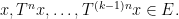
Let us first explain what a finite extension is. Given a measure-preserving system {X = (X,{\mathcal X},\mu,T)}, a finite set {Y}, and a measurable map {\rho: X \rightarrow \hbox{Sym}(Y)} from {X} to the permutation group of {Y}, one can form the finite extension

\displaystyle X \ltimes_\rho Y = (X \times Y, {\mathcal X} \times {\mathcal Y}, \mu \times \nu, S),

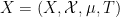
which as a probability space is the product of {(X,{\mathcal X},\mu)} with the finite probability space {Y = (Y, {\mathcal Y},\nu)} (with the discrete {\sigma}-algebra and uniform probability measure), and with shift map

\displaystyle  S(x, y) := (Tx, \rho(x) y). \ \ \ \ \ (1)

One easily verifies that this is indeed a measure-preserving system. We refer to {\rho} as the cocycle of the system.

An example of finite extensions comes from group theory. Suppose we have a short exact sequence

\displaystyle  0 \rightarrow K \rightarrow G \rightarrow H \rightarrow 0

of finite groups. Let {g} be a group element of {G}, and let {h} be its projection in {H}. Then the shift map {x \mapsto gx} on {G} (with the discrete {\sigma}-algebra and uniform probability measure) can be viewed as a finite extension of the shift map {y \mapsto hy} on {H} (again with the discrete {\sigma}-algebra and uniform probability measure), by arbitrarily selecting a section {\phi: H \rightarrow G} that inverts the projection map, identifying {G} with {H \times K} by identifying {k \phi(y)} with {(y,k)} for {y \in H, k \in K}, and using the cocycle

\displaystyle  \rho(y) := \phi(hy)^{-1} g \phi(y).

Thus, for instance, the unit shift {x \mapsto x+1} on {{\bf Z}/N{\bf Z}} can be thought of as a finite extension of the unit shift {x \mapsto x+1} on {{\bf Z}/M{\bf Z}} whenever {N} is a multiple of {M}.

Another example comes from Riemannian geometry. If {M} is a Riemannian manifold that is a finite cover of another Riemannian manifold {N} (with the metric on {M} being the pullback of that on {N}), then (unit time) geodesic flow on the cosphere bundle of {M} is a finite extension of the corresponding flow on {N}.

Here, then, is the finite extension special case of the compact extension step in the proof of the multiple recurrence theorem:

Proposition 2 (Finite extensions) Let {X \rtimes_\rho Y} be a finite extension of a measure-preserving system {X}. If {X} obeys the conclusion of the Furstenberg multiple recurrence theorem, then so does {X \rtimes_\rho Y}.

Before we prove this proposition, let us first give the combinatorial analogue.

Lemma 3 Let {A} be a subset of the integers that contains arbitrarily long arithmetic progressions, and let {A = A_1 \cup \ldots \cup A_M} be a colouring of {A} by {M} colours (or equivalently, a partition of {A} into {M} colour classes {A_i}). Then at least one of the {A_i} contains arbitrarily long arithmetic progressions.

Proof: By the infinite pigeonhole principle, it suffices to show that for each {k \geq 1}, one of the colour classes {A_i} contains an arithmetic progression of length {k}.

Let {N} be a large integer (depending on {k} and {M}) to be chosen later. Then {A} contains an arithmetic progression of length {N}, which may be identified with {\{0,\ldots,N-1\}}. The colouring of {A} then induces a colouring on {\{0,\ldots,N-1\}} into {M} colour classes. Applying (the finitary form of) van der Waerden’s theorem, we conclude that if {N} is sufficiently large depending on {M} and {k}, then one of these colouring classes contains an arithmetic progression of length {k}; undoing the identification, we conclude that one of the {A_i} contains an arithmetic progression of length {k}, as desired. \Box

Of course, by specialising to the case {A={\bf Z}}, we see that the above Lemma is in fact equivalent to van der Waerden’s theorem.

Now we prove Proposition 2.

Proof: Fix {k}. Let {E} be a positive measure subset of {X \rtimes_\rho Y = (X \times Y, {\mathcal X} \times {\mathcal Y}, \mu \times \nu, S)}. By Fubini’s theorem, we have

\displaystyle  \mu \times \nu(E) = \int_X f(x)\ d\mu(x)

where {f(x) := \nu(E_x)} and {E_x := \{ y \in Y: (x,y) \in E \}} is the fibre of {E} at {x}. Since {\mu \times \nu(E)} is positive, we conclude that the set

\displaystyle F := \{ x \in X: f(x) > 0 \} = \{ x \in X: E_x \neq \emptyset \}

is a positive measure subset of {X}. Note for each {x \in F}, we can find an element {g(x) \in Y} such that {(x,g(x)) \in E}. While not strictly necessary for this argument, one can ensure if one wishes that the function {g} is measurable by totally ordering {Y}, and then letting {g(x)} the minimal element of {Y} for which {(x,g(x)) \in E}.

Let {N} be a large integer (which will depend on {k} and the cardinality {M} of {Y}) to be chosen later. Because {X} obeys the multiple recurrence theorem, we can find a positive integer {n} and {x \in X} such that

\displaystyle  x, T^n x, T^{2n} x, \ldots, T^{(N-1) n} x \in F.

Now consider the sequence of {N} points

\displaystyle  S^{-mn}( T^{mn} x, g(T^{mn} x) )

for {m = 0,\ldots,N-1}. From (1), we see that

\displaystyle  S^{-mn}( T^{mn} x, g(T^{mn} x) ) = (x, c(m)) \ \ \ \ \ (2)

for some sequence {c(0),\ldots,c(N-1) \in Y}. This can be viewed as a colouring of {\{0,\ldots,N-1\}} by {M} colours, where {M} is the cardinality of {Y}. Applying van der Waerden’s theorem, we conclude (if {N} is sufficiently large depending on {k} and {|Y|}) that there is an arithmetic progression {a, a+r,\ldots,a+(k-1)r} in {\{0,\ldots,N-1\}} with {r>0} such that

\displaystyle  c(a) = c(a+r) = \ldots = c(a+(k-1)r) = c

for some {c \in Y}. If we then let {y = (x,c)}, we see from (2) that

\displaystyle  S^{an + irn} y = ( T^{(a+ir)n} x, g(T^{(a+ir)n} x) ) \in E

for all {i=0,\ldots,k-1}, and the claim follows. \Box

Remark 1 The precise connection between Lemma 3 and Proposition 2 arises from the following observation: with {E, F, g} as in the proof of Proposition 2, and {x \in X}, the set

\displaystyle  A := \{ n \in {\bf Z}: T^n x \in F \}

can be partitioned into the classes

\displaystyle  A_i := \{ n \in {\bf Z}: S^n (x,i) \in E' \}

where {E' := \{ (x,g(x)): x \in F \} \subset E} is the graph of {g}. The multiple recurrence property for {X} ensures that {A} contains arbitrarily long arithmetic progressions, and so therefore one of the {A_i} must also, which gives the multiple recurrence property for {Y}.

Remark 2 Compact extensions can be viewed as a generalisation of finite extensions, in which the fibres are no longer finite sets, but are themselves measure spaces obeying an additional property, which roughly speaking asserts that for many functions {f} on the extension, the shifts {T^n f} of {f} behave in an almost periodic fashion on most fibres, so that the orbits {T^n f} become totally bounded on each fibre. This total boundedness allows one to obtain an analogue of the above colouring map {c()} to which van der Waerden’s theorem can be applied.

Archives