
You are currently browsing the tag archive for the ‘nilsequences’ tag.
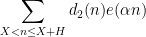
Kaisa Matomäki, Xuancheng Shao, Joni Teräväinen, and myself have just uploaded to the arXiv our preprint “Higher uniformity of arithmetic functions in short intervals I. All intervals“. This paper investigates the higher order (Gowers) uniformity of standard arithmetic functions in analytic number theory (and specifically, the Möbius function 


![{(X,X+H]}](https://s0.wp.com/latex.php?latex=%7B%28X%2CX%2BH%5D%7D&bg=ffffff&fg=000000&s=0&c=20201002)


 , where
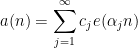
  . For applications in the additive combinatorics of such functions , it is also necessary to consider more general correlations, such as polynomial correlations
 is a polynomial of some fixed degree, or more generally
 is a nilmanifold of fixed degree and dimension (and with some control on structure constants),
  is a polynomial map, and
  is a Lipschitz function (with some bound on the Lipschitz constant). Indeed, thanks to the inverse theorem for the Gowers uniformity norm, such correlations let one control the Gowers uniformity norm of (possibly after subtracting off some renormalising factor) on such short intervals , which can in turn be used to control other multilinear correlations involving such functions.
Traditionally, asymptotics for such sums are expressed in terms of a “main term” of some arithmetic nature, plus an error term that is estimated in magnitude. For instance, a sum such as 

 variable to be restricted further to a subprogression of , but let us ignore this minor extension for this discussion). There is some flexibility in how to choose these approximants, but we eventually found it convenient to use the following choices.
- For the Möbius function
, as per the Möbius pseudorandomness conjecture. (One could choose a more sophisticated approximant in the presence of a Siegel zero, as I did with Joni in this recent paper, but we do not do so here.)
- For the von Mangoldt function
, where
and
.
- For the divisor functions
for some explicit polynomials
, chosen so that
and
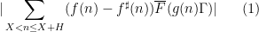
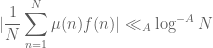
The objective is then to obtain bounds on sums such as (1) that improve upon the “trivial bound” that one can get with the triangle inequality and standard number theory bounds such as the Brun-Titchmarsh inequality. For 


Our main estimates on sums of the form (1) work in the following ranges:
- For
, one can obtain strongly logarithmic savings on (1) for
, and power savings for
.
- For
, one can obtain weakly logarithmic savings for
.
- For
, one can obtain power savings for
.
- For
, one can obtain power savings for
.
Conjecturally, one should be able to obtain power savings in all cases, and lower 

By combining these results with tools from additive combinatorics, one can obtain a number of applications:
- Direct insertion of our bounds in the recent work of Kanigowski, Lemanczyk, and Radziwill on the prime number theorem on dynamical systems that are analytic skew products gives some improvements in the exponents there.
- We can obtain a “short interval” version of a multiple ergodic theorem along primes established by Frantzikinakis-Host-Kra and Wooley-Ziegler, in which we average over intervals of the form
.
- We can obtain a “short interval” version of the “linear equations in primes” asymptotics obtained by Ben Green, Tamar Ziegler, and myself in this sequence of papers, where the variables in these equations lie in short intervals
We now briefly discuss some of the ingredients of proof of our main results. The first step is standard, using combinatorial decompositions (based on the Heath-Brown identity and (for the 
- Type
sums, which are basically of the form
for some weights
of controlled size and some cutoff
that is not too large;
- Type
sums, which are basically of the form
for some weights
of controlled size and some cutoffs
that are not too close to
or to
- Type
sums, which are basically of the form
for some weights
The precise ranges of the cutoffs 
The Type
For the Type 


 range in various dyadic intervals. Using the known multidimensional equidistribution theory of polynomial maps in nilmanifolds, one can eventually show in the non-abelian case that this sequence either has enough equidistribution to give cancellation, or else the nilsequence involved can be replaced with one from a lower dimensional nilmanifold, in which case one can apply an induction hypothesis.
For the type

 into a number of arithmetic progressions, and then uses equidistribution theory to establish cancellation of sequences such as
  on the majority of these progressions. As it turns out, this strategy works well in the regime
  unless the nilsequence involved is “major arc”, but the latter case is treatable by existing methods as discussed previously; this is why the exponent for our
  result can be as low as
  .
.
In a sequel to this paper (currently in preparation), we will obtain analogous results for almost all intervals ![{(x,x+H]}](https://s0.wp.com/latex.php?latex=%7B%28x%2Cx%2BH%5D%7D&bg=ffffff&fg=000000&s=0&c=20201002)

![{[X,2X]}](https://s0.wp.com/latex.php?latex=%7B%5BX%2C2X%5D%7D&bg=ffffff&fg=000000&s=0&c=20201002)

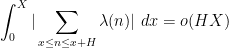
Kaisa Matomäki, Maksym Radziwill, Joni Teräväinen, Tamar Ziegler and I have uploaded to the arXiv our paper Higher uniformity of bounded multiplicative functions in short intervals on average. This paper (which originated from a working group at an AIM workshop on Sarnak’s conjecture) focuses on the local Fourier uniformity conjecture for bounded multiplicative functions such as the Liouville function 
![\displaystyle \int_0^X \| \lambda \|_{U^k([x,x+H])}\ dx = o(X) \ \ \ \ \ (1)](https://s0.wp.com/latex.php?latex=%5Cdisplaystyle++%5Cint_0%5EX+%5C%7C+%5Clambda+%5C%7C_%7BU%5Ek%28%5Bx%2Cx%2BH%5D%29%7D%5C+dx+%3D+o%28X%29+%5C+%5C+%5C+%5C+%5C+%281%29&bg=ffffff&fg=000000&s=0&c=20201002)
 for any fixed
  and any
 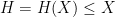 that goes to infinity as , where
 ![{U^k([x,x+H])}](https://s0.wp.com/latex.php?latex=%7BU%5Ek%28%5Bx%2Cx%2BH%5D%29%7D&bg=ffffff&fg=000000&s=0&c=20201002) is the (normalized) Gowers uniformity norm. Among other things this conjecture implies (logarithmically averaged version of) the Chowla and Sarnak conjectures for the Liouville function (or the Möbius function), see this previous blog post.
is the (normalized) Gowers uniformity norm. Among other things this conjecture implies (logarithmically averaged version of) the Chowla and Sarnak conjectures for the Liouville function (or the Möbius function), see this previous blog post.
The conjecture gets more difficult as 

 ) in a landmark paper of Matomäki and Radziwill, discussed for instance in this blog post.
For 
 (and it would be a major breakthrough in particular if one could obtain this bound for as small as
  for any fixed
  , particularly if applicable to more general bounded multiplicative functions than , as this would have new implications for a generalization of the Chowla conjecture known as the Elliott conjecture). Recently, Kaisa, Maks and myself were able to establish this conjecture in the range
  (in fact we have since worked out in the current paper that we can get as small as
  ). In our current paper we establish Fourier uniformity conjecture for higher for the same range of . This in particular implies local orthogonality to polynomial phases,
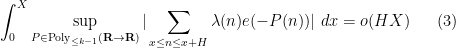
 denotes the polynomials of degree at most
  , but the full conjecture is a bit stronger than this, establishing the more general statement
 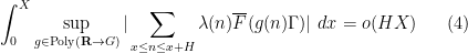 filtered nilmanifold and Lipschitz function , where
  now ranges over polynomial maps from
  to . The method of proof follows the same general strategy as in the previous paper with Kaisa and Maks. (The equivalence of (4) and (1) follows from the inverse conjecture for the Gowers norms, proven in this paper.) We quickly sketch first the proof of (3), using very informal language to avoid many technicalities regarding the precise quantitative form of various estimates. If the estimate (3) fails, then we have the correlation estimate
 and some polynomial
  depending on . The difficulty here is to understand how can depend on . We write the above correlation estimate more suggestively as
 ![\displaystyle \lambda(n) \sim_{[x,x+H]} e(P_x(n)).](https://s0.wp.com/latex.php?latex=%5Cdisplaystyle++%5Clambda%28n%29+%5Csim_%7B%5Bx%2Cx%2BH%5D%7D+e%28P_x%28n%29%29.&bg=ffffff&fg=000000&s=0&c=20201002)
 at small primes
  , one expects to have a relation of the form
 ![\displaystyle e(P_{x'}(p'n)) \sim_{[x/p,x/p+H/p]} e(P_x(pn)) \ \ \ \ \ (5)](https://s0.wp.com/latex.php?latex=%5Cdisplaystyle++e%28P_%7Bx%27%7D%28p%27n%29%29+%5Csim_%7B%5Bx%2Fp%2Cx%2Fp%2BH%2Fp%5D%7D+e%28P_x%28pn%29%29+%5C+%5C+%5C+%5C+%5C+%285%29&bg=ffffff&fg=000000&s=0&c=20201002)
 for which
  for some small primes
  . (This can be formalised using an inequality of Elliott related to the Turan-Kubilius theorem.) This gives a relationship between and
  for “edges” in a rather sparse “graph” connecting the elements of say
 ![{[X/2,X]}](https://s0.wp.com/latex.php?latex=%7B%5BX%2F2%2CX%5D%7D&bg=ffffff&fg=000000&s=0&c=20201002) . Using some graph theory one can locate some non-trivial “cycles” in this graph that eventually lead (in conjunction to a certain technical but important “Chinese remainder theorem” step to modify the to eliminate a rather serious “aliasing” issue that was already discussed in this previous post) to obtain functional equations of the form
. Using some graph theory one can locate some non-trivial “cycles” in this graph that eventually lead (in conjunction to a certain technical but important “Chinese remainder theorem” step to modify the to eliminate a rather serious “aliasing” issue that was already discussed in this previous post) to obtain functional equations of the form 
 , where
  should be viewed as a first approximation (ignoring a certain “profinite” or “major arc” term for simplicity) as “differing by a slowly varying polynomial” and the polynomials should now be viewed as taking values on the reals rather than the integers. This functional equation can be solved to obtain a relation of the form
 of polynomial size, and with further analysis of the relation (5) one can make basically independent of . This simplifies (3) to something like
 is a bounded multiplicative function). (Actually because of the profinite term mentioned previously, one also has to insert a Dirichlet character of bounded conductor into this latter conclusion, but we will ignore this technicality.)
Now we apply the same strategy to (4). For abelian 
 is rather technical and will not be detailed here. A new difficulty arises in that there are some unwanted solutions to this equation, such as
 , which do not necessarily lead to multiplicative characters like
  as in the polynomial case, but instead to some unfriendly looking “generalized multiplicative characters” (think of
  as a rough caricature). To avoid this problem, we rework the graph theory portion of the argument to produce not just one functional equation of the form (6)for each , but many, leading to dilation invariances
  . From a certain amount of Lie algebra theory (ultimately arising from an understanding of the behaviour of the exponential map on nilpotent matrices, and exploiting the hypothesis that is non-abelian) one can conclude that (after some initial preparations to avoid degenerate cases)
  must behave like
  for some central element
  of . This eventually brings one back to the multiplicative characters that arose in the polynomial case, and the arguments now proceed as before.
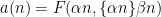
We give two applications of this higher order Fourier uniformity. One regards the growth of the number
 sign patterns in the Liouville function. The Chowla conjecture implies that
  , but even the weaker conjecture of Sarnak that
  for some remains open. Until recently, the best asymptotic lower bound on
  was
was  , due to McNamara; with our result, we can now show
  for any (in fact we can get
  for any ). The idea is to repeat the now-standard argument to exploit multiplicativity at small primes to deduce Chowla-type conjectures from Fourier uniformity conjectures, noting that the Chowla conjecture would give all the sign patterns one could hope for. The usual argument here uses the “entropy decrement argument” to eliminate a certain error term (involving the large but mean zero factor
  ). However the observation is that if there are extremely few sign patterns of length , then the entropy decrement argument is unnecessary (there isn’t much entropy to begin with), and a more low-tech moment method argument (similar to the derivation of Chowla’s conjecture from Sarnak’s conjecture, as discussed for instance in this post) gives enough of Chowla’s conjecture to produce plenty of length sign patterns. If there are not extremely few sign patterns of length then we are done anyway. One quirk of this argument is that the sign patterns it produces may only appear exactly once; in contrast with preceding arguments, we were not able to produce a large number of sign patterns that each occur infinitely often.
The second application is to obtain cancellation for various polynomial averages involving the Liouville function


 are polynomials of degree at most
  , no two of which differ by a constant (the latter is essential to avoid having to establish the Chowla or Hardy-Littlewood conjectures, which of course remain open). Results of this type were previously obtained by Tamar Ziegler and myself in the “true complexity zero” case when the polynomials
  had distinct degrees, in which one could use the theory of Matomäki and Radziwill; now that higher is available at the scale
  we can now remove this restriction.
A sequence 

for some real numbers 


with 

These sequences arise in various “complexity one” problems in arithmetic combinatorics and ergodic theory. For instance, if 


can be shown to be an almost periodic sequence, plus an error term 

This can be established in a number of ways, for instance by writing 


In the last two decades or so, it has become clear that there are natural higher order versions of these concepts, in which linear polynomials such as 


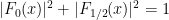
For technical reasons (having to do with the non-trivial topological structure on nilmanifolds), it will be convenient to work with vector-valued sequences, that take values in a finite-dimensional complex vector space 


This product is associative and bilinear, and also commutative up to permutation of the indices. It also interacts well with the Hermitian norm

since we have 
The traditional definition of a basic nilsequence (as defined for instance by Bergelson, Host, and Kra) is as follows:
Definition 1 (Basic nilsequence, first definition) A nilmanifold of step at most
-fold commutators vanish) and
is a discrete cocompact lattice in
, where
,
, and
is a continuous function.
For instance, it is not difficult using this definition to show that a sequence is a basic nilsequence of degree at most 
Nowadays, and particularly when one needs to understand the “single-scale” equidistribution properties of nilsequences, it is more convenient (as is for instance done in this ICM paper of Green) to use an alternate definition of a nilsequence as follows.
Definition 2 Let
. A filtered group of degree at most
of subgroups
with
and
for
. A polynomial sequence
for all
and
, where
is the difference operator. A filtered nilmanifold of degree at most
is a quotient
are connected, simply connected nilpotent filtered Lie group, and
is a discrete cocompact subgroup of
, where
is a continuous function which is
for all
One can easily identify a 

It is easy to see that any sequence that is a basic nilsequence of degree at most 

where 


The other key example is a sequence of the form
where 


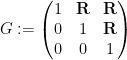
with the lower central series filtration 
![{G_2= [G,G] = \begin{pmatrix} 1 &0 & {\bf R} \\ 0 & 1 & 0 \\ 0 & 0 & 1 \end{pmatrix}}](https://s0.wp.com/latex.php?latex=%7BG_2%3D+%5BG%2CG%5D+%3D+%5Cbegin%7Bpmatrix%7D+1+%260+%26+%7B%5Cbf+R%7D+%5C%5C+0+%26+1+%26+0+%5C%5C+0+%26+0+%26+1+%5Cend%7Bpmatrix%7D%7D&bg=ffffff&fg=000000&s=0&c=20201002)


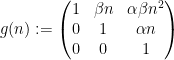
and 

one easily verifies that this function is indeed 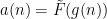


will be a basic nilsequence if 
A nilsequence of degree at most 


is equal to a nilsequence of degree at most 

It is easy to see that a sequence 


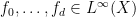
Now we turn to the notion of a nilcharacter, as defined in this paper of Ben Green, Tamar Ziegler, and myself:
Definition 3 (Nilcharacters) Let
. A sub-nilcharacter of degree
of degree at most
for all
, where
is a continuous homomorphism
. (Note from (1) and
must map
to
.) If in addition one has
for all

In the degree one case 


where 

for all 


We claim that every degree 


and then

becomes a degree 
As we shall show below, nilsequences can be approximated uniformly by linear combinations of nilcharacters, in much the same way that quasiperiodic or almost periodic sequences can be approximated uniformly by linear combinations of linear phases. In particular, nilcharacters can be used as “obstructions to uniformity” in the sense of the inverse theory of the Gowers uniformity norms.
The space of degree
Definition 4 Let
,
are equivalent if
is equal (as a sequence) to a basic nilsequence of degree at most
of such a nilcharacter will be called the symbol of that nilcharacter (in analogy to the symbol of a differential or pseudodifferential operator), and the collection of such symbols will be denoted
.
As we shall see below the fold, 


Note: this post is of a particularly technical nature, in particular presuming familiarity with nilsequences, nilsystems, characteristic factors, etc., and is primarily intended for experts.
As mentioned in the previous post, Ben Green, Tamar Ziegler, and myself proved the following inverse theorem for the Gowers norms:
Theorem 1 (Inverse theorem for Gowers norms) Let
and
be integers, and let
. Suppose that
is a function supported on
such that
Then there exists a filtered nilmanifold
and complexity
, a polynomial sequence
of Lipschitz constant

This result was conjectured earlier by Ben Green and myself; this conjecture was strongly motivated by an analogous inverse theorem in ergodic theory by Host and Kra, which we formulate here in a form designed to resemble Theorem 1 as closely as possible:
Theorem 2 (Inverse theorem for Gowers-Host-Kra seminorms) Let
be an ergodic, countably generated measure-preserving system. Suppose that one has
for all non-zero
(all
spaces are real-valued in this post). Then
is an inverse limit (in the category of measure-preserving systems, up to almost everywhere equivalence) of ergodic degree
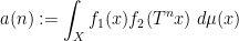
for some degree
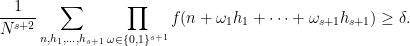
![\displaystyle \lim_{N \rightarrow \infty} \frac{1}{N^{s+1}} \sum_{h_1,\dots,h_{s+1} \in [N]} \int_X \prod_{\omega \in \{0,1\}^{s+1}} f(T^{\omega_1 h_1 + \dots + \omega_{s+1} h_{s+1}}x)\ d\mu(x)](https://s0.wp.com/latex.php?latex=%5Cdisplaystyle+%5Clim_%7BN+%5Crightarrow+%5Cinfty%7D+%5Cfrac%7B1%7D%7BN%5E%7Bs%2B1%7D%7D+%5Csum_%7Bh_1%2C%5Cdots%2Ch_%7Bs%2B1%7D+%5Cin+%5BN%5D%7D+%5Cint_X+%5Cprod_%7B%5Comega+%5Cin+%5C%7B0%2C1%5C%7D%5E%7Bs%2B1%7D%7D+f%28T%5E%7B%5Comega_1+h_1+%2B+%5Cdots+%2B+%5Comega_%7Bs%2B1%7D+h_%7Bs%2B1%7D%7Dx%29%5C+d%5Cmu%28x%29+&bg=ffffff&fg=000000&s=0&c=20201002)

It is a natural question to ask if there is any logical relationship between the two theorems. In the finite field category, one can deduce the combinatorial inverse theorem from the ergodic inverse theorem by a variant of the Furstenberg correspondence principle, as worked out by Tamar Ziegler and myself, however in the current context of
One can split Theorem 2 into two components:
Theorem 3 (Weak inverse theorem for Gowers-Host-Kra seminorms) Let
for all non-zero
. Then
![\displaystyle \lim_{N \rightarrow \infty} \frac{1}{N^{s+1}} \sum_{h_1,\dots,h_{s+1} \in [N]} \int_X \prod_{\omega \in \{0,1\}^{s+1}} T^{\omega_1 h_1 + \dots + \omega_{s+1} h_{s+1}} f\ d\mu](https://s0.wp.com/latex.php?latex=%5Cdisplaystyle+%5Clim_%7BN+%5Crightarrow+%5Cinfty%7D+%5Cfrac%7B1%7D%7BN%5E%7Bs%2B1%7D%7D+%5Csum_%7Bh_1%2C%5Cdots%2Ch_%7Bs%2B1%7D+%5Cin+%5BN%5D%7D+%5Cint_X+%5Cprod_%7B%5Comega+%5Cin+%5C%7B0%2C1%5C%7D%5E%7Bs%2B1%7D%7D+T%5E%7B%5Comega_1+h_1+%2B+%5Cdots+%2B+%5Comega_%7Bs%2B1%7D+h_%7Bs%2B1%7D%7D+f%5C+d%5Cmu&bg=ffffff&fg=000000&s=0&c=20201002)
Theorem 4 (Pro-nilsystems closed under factors) Let
Indeed, it is clear that Theorem 2 implies both Theorem 3 and Theorem 4, and conversely that the two latter theorems jointly imply the former. Theorem 4 is, in principle, purely a fact about nilsystems, and should have an independent proof, but this is not known; the only known proofs go through the full machinery needed to prove Theorem 2 (or the closely related theorem of Ziegler). (However, the fact that a factor of a nilsystem is again a nilsystem was established previously by Parry.)
The purpose of this post is to record a partial implication in reverse direction to the correspondence principle:
As mentioned at the start of the post, a fair amount of familiarity with the area is presumed here, and some routine steps will be presented with only a fairly brief explanation.
One of the basic objects of study in combinatorics are finite strings 


On the other hand, the basic object of study in dynamics (and in related fields, such as ergodic theory) is that of a dynamical system 


There is a fundamental correspondence principle connecting the study of strings (or subsets of natural numbers or integers) with the study of dynamical systems. In one direction, given a dynamical system 


Example 1 If
with the shift map
,
is the observable that takes the value
and zero at the other two classes, and one starts with the initial datum
, then the observed string
In the converse direction, every infinite string 

let

and let

Then one easily sees that the observed string 


In the case when the alphabet 


The above universal construction is very easy to describe, and is well suited for “generic” strings 
A related aesthetic objection to the universal construction is that of the four components 

One step in this direction can be made by restricting 


For general sequences
In Notes 5, we saw that the Gowers uniformity norms on vector spaces 

Now we study the analogous situation on cyclic groups 

Traditionally, nilsequences have been defined in terms of linear orbits 

A polynomial phase 


In these notes we set out the basic theory for these nilsequences, including their equidistribution theory (which generalises the equidistribution theory of polynomial flows on tori from Notes 1) and show that they are indeed obstructions to the Gowers norm being small. This leads to the inverse conjecture for the Gowers norms that shows that the Gowers norms on cyclic groups are indeed controlled by these sequences.
Ben Green, and I have just uploaded to the arXiv our paper “An arithmetic regularity lemma, an associated counting lemma, and applications“, submitted (a little behind schedule) to the 70th birthday conference proceedings for Endre Szemerédi. In this paper we describe the general-degree version of the arithmetic regularity lemma, which can be viewed as the counterpart of the Szemerédi regularity lemma, in which the object being regularised is a function ![{f: [N] \rightarrow [0,1]}](https://s0.wp.com/latex.php?latex=%7Bf%3A+%5BN%5D+%5Crightarrow+%5B0%2C1%5D%7D&bg=ffffff&fg=000000&s=0&c=20201002)
![{[N] = \{1,\ldots,N\}}](https://s0.wp.com/latex.php?latex=%7B%5BN%5D+%3D+%5C%7B1%2C%5Cldots%2CN%5C%7D%7D&bg=ffffff&fg=000000&s=0&c=20201002)

![{U^{s+1}[N]}](https://s0.wp.com/latex.php?latex=%7BU%5E%7Bs%2B1%7D%5BN%5D%7D&bg=ffffff&fg=000000&s=0&c=20201002)
The regularity lemma is a manifestation of the “dichotomy between structure and randomness”, as discussed for instance in my ICM article or FOCS article. In the degree 

The regularity and counting lemmas are designed to be used together, and in the paper we give three applications of this combination. Firstly, we give a new proof of Szemerédi’s theorem, which proceeds via an energy increment argument rather than a density increment one. Secondly, we establish a conjecture of Bergelson, Host, and Kra, namely that if ![{A \subset [N]}](https://s0.wp.com/latex.php?latex=%7BA+%5Csubset+%5BN%5D%7D&bg=ffffff&fg=000000&s=0&c=20201002)


![{[N]}](https://s0.wp.com/latex.php?latex=%7B%5BN%5D%7D&bg=ffffff&fg=000000&s=0&c=20201002)
In all three applications, the scheme of proof can be described as follows:
- Apply the arithmetic regularity lemma, and decompose a relevant function
.
- The uniform part
is so tiny in the Gowers uniformity norm that its contribution can be easily dealt with by an appropriate “generalised von Neumann theorem”.
- The contribution of the (virtual, irrational) nilsequence
can be controlled using the arithmetic counting lemma.
- Finally, one needs to check that the contribution of the small error
does not overwhelm the main term
To illustrate the last point, let us give the following example. Suppose we have a set 


Unfortunately, the answer could be no; conceivably, all of the 

But suppose we knew that the 

A succinct (but slightly inaccurate) summation of the regularity+counting lemma strategy would be that in order to solve a problem in additive combinatorics, it “suffices to check it for nilsequences”. But this should come with a caveat, due to the issue of the small error above; in addition to checking it for nilsequences, the answer in the nilsequence case must be sufficiently “dispersed” in a suitable sense, so that it can survive the addition of a small (but not completely negligible) perturbation.
One last “production note”. Like our previous paper with Emmanuel Breuillard, we used Subversion to write this paper, which turned out to be a significant efficiency boost as we could work on different parts of the paper simultaneously (this was particularly important this time round as the paper was somewhat lengthy and complicated, and there was a submission deadline). When doing so, we found it convenient to split the paper into a dozen or so pieces (one for each section of the paper, basically) in order to avoid conflicts, and to help coordinate the writing process. I’m also looking into git (a more advanced version control system), and am planning to use it for another of my joint projects; I hope to be able to comment on the relative strengths of these systems (and with plain old email) in the future.
Ben Green and I have just uploaded to the arXiv our paper, “The Möbius function is asymptotically orthogonal to nilsequences“, which is a sequel to our earlier paper “The quantitative behaviour of polynomial orbits on nilmanifolds“, which I talked about in this post. In this paper, we apply our previous results on quantitative equidistribution polynomial orbits in nilmanifolds to settle the Möbius and nilsequences conjecture from our earlier paper, as part of our program to detect and count solutions to linear equations in primes. (The other major plank of that program, namely the inverse conjecture for the Gowers norm, remains partially unresolved at present.) Roughly speaking, this conjecture asserts the asymptotic orthogonality
between the Möbius function 


There is an amusing way to interpret the conjecture (using the close relationship between nilsequences and bracket polynomials) as an assertion of the pseudorandomness of the Liouville function from a computational complexity perspective. Suppose you possess a calculator with the wonderful property of being infinite precision: it can accept arbitrarily large real numbers as input, manipulate them precisely, and also store them in memory. However, this calculator has two limitations. Firstly, the only operations available are addition, subtraction, multiplication, integer part ![x \mapsto [x]](https://s0.wp.com/latex.php?latex=x+%5Cmapsto+%5Bx%5D&bg=ffffff&fg=545454&s=0&c=20201002)


Now suppose you play the following game with an opponent.
- The opponent specifies a large integer d.
- You get to enter in O(1) real constants of your choice into your calculator. These can be absolute constants such as
and
, or they can depend on d (e.g. you can enter in
).
- The opponent randomly selects an d-digit integer n, and enters n into one of the registers of your calculator.
- You are allowed to perform O(1) operations on your calculator and record what is displayed on the calculator’s viewscreen.
- After this, you have to guess whether the opponent’s number n had an odd or even number of prime factors (i.e. you guess
.)
- If you guess correctly, you win $1; otherwise, you lose $1.
For instance, using your calculator you can work out the first few digits of 


Our theorem is equivalent to the assertion that as d goes to infinity (keeping the O(1) constants fixed), your probability of winning this game converges to 1/2; in other words, your calculator becomes asymptotically useless to you for the purposes of guessing whether n has an odd or even number of prime factors, and you may as well just guess randomly.
[I should mention a recent result in a similar spirit by Mauduit and Rivat; in this language, their result asserts that knowing the last few digits of the digit-sum of n does not increase your odds of guessing

Recent Comments