
You are currently browsing the monthly archive for February 2013.
The following result is due independently to Furstenberg and to Sarkozy:
Theorem 1 (Furstenberg-Sarkozy theorem) Let
, and suppose that
is sufficiently large depending on
. Then every subset
of
of density
at least
for some natural numbers
with
.
This theorem is of course similar in spirit to results such as Roth’s theorem or Szemerédi’s theorem, in which the pattern 


A few years ago, Ben Green, Tamar Ziegler, and myself observed that it is possible to prove the Furstenberg-Sarkozy theorem by just using the Cauchy-Schwarz inequality (or van der Corput lemma) and the density increment argument, removing all invocations of Fourier analysis, and instead relying on Cauchy-Schwarz to linearise the quadratic shift 
The first step is to use the density increment argument that goes back to Roth. For any 
![{A \subset [N]}](https://s0.wp.com/latex.php?latex=%7BA+%5Csubset+%5BN%5D%7D&bg=ffffff&fg=000000&s=0&c=20201002)


for some absolute constant 

It remains to establish the implication (1). Suppose for sake of contradiction that we can find 

![{[N]}](https://s0.wp.com/latex.php?latex=%7B%5BN%5D%7D&bg=ffffff&fg=000000&s=0&c=20201002)

![\displaystyle \mathop{\bf E}_{n \in [N]} \mathop{\bf E}_{r \in [N^{1/3}]} \mathop{\bf E}_{h \in [N^{1/100}]} 1_A(n) 1_A(n+(r+h)^2) = 0.](https://s0.wp.com/latex.php?latex=%5Cdisplaystyle++%5Cmathop%7B%5Cbf+E%7D_%7Bn+%5Cin+%5BN%5D%7D+%5Cmathop%7B%5Cbf+E%7D_%7Br+%5Cin+%5BN%5E%7B1%2F3%7D%5D%7D+%5Cmathop%7B%5Cbf+E%7D_%7Bh+%5Cin+%5BN%5E%7B1%2F100%7D%5D%7D+1_A%28n%29+1_A%28n%2B%28r%2Bh%29%5E2%29+%3D+0.&bg=ffffff&fg=000000&s=0&c=20201002)
(The exact ranges of 
Let 

![\displaystyle \mathop{\bf E}_{n \in [N]} \mathop{\bf E}_{r \in [N^{1/3}]} \mathop{\bf E}_{h \in [N^{1/100}]} 1_A(n) \delta 1_{[N]}(n+(r+h)^2) = \delta^2 + O(N^{-1/3})](https://s0.wp.com/latex.php?latex=%5Cdisplaystyle++%5Cmathop%7B%5Cbf+E%7D_%7Bn+%5Cin+%5BN%5D%7D+%5Cmathop%7B%5Cbf+E%7D_%7Br+%5Cin+%5BN%5E%7B1%2F3%7D%5D%7D+%5Cmathop%7B%5Cbf+E%7D_%7Bh+%5Cin+%5BN%5E%7B1%2F100%7D%5D%7D+1_A%28n%29+%5Cdelta+1_%7B%5BN%5D%7D%28n%2B%28r%2Bh%29%5E2%29+%3D+%5Cdelta%5E2+%2B+O%28N%5E%7B-1%2F3%7D%29&bg=ffffff&fg=000000&s=0&c=20201002)
![\displaystyle \mathop{\bf E}_{n \in [N]} \mathop{\bf E}_{r \in [N^{1/3}]} \mathop{\bf E}_{h \in [N^{1/100}]} \delta 1_{[N]}(n) \delta 1_{[N]}(n+(r+h)^2) = \delta^2 + O(N^{-1/3})](https://s0.wp.com/latex.php?latex=%5Cdisplaystyle++%5Cmathop%7B%5Cbf+E%7D_%7Bn+%5Cin+%5BN%5D%7D+%5Cmathop%7B%5Cbf+E%7D_%7Br+%5Cin+%5BN%5E%7B1%2F3%7D%5D%7D+%5Cmathop%7B%5Cbf+E%7D_%7Bh+%5Cin+%5BN%5E%7B1%2F100%7D%5D%7D+%5Cdelta+1_%7B%5BN%5D%7D%28n%29+%5Cdelta+1_%7B%5BN%5D%7D%28n%2B%28r%2Bh%29%5E2%29+%3D+%5Cdelta%5E2+%2B+O%28N%5E%7B-1%2F3%7D%29&bg=ffffff&fg=000000&s=0&c=20201002)
and
![\displaystyle \mathop{\bf E}_{n \in [N]} \mathop{\bf E}_{r \in [N^{1/3}]} \mathop{\bf E}_{h \in [N^{1/100}]} \delta 1_{[N]}(n) 1_A(n+(r+h)^2) = \delta^2 + O( N^{-1/3} ).](https://s0.wp.com/latex.php?latex=%5Cdisplaystyle++%5Cmathop%7B%5Cbf+E%7D_%7Bn+%5Cin+%5BN%5D%7D+%5Cmathop%7B%5Cbf+E%7D_%7Br+%5Cin+%5BN%5E%7B1%2F3%7D%5D%7D+%5Cmathop%7B%5Cbf+E%7D_%7Bh+%5Cin+%5BN%5E%7B1%2F100%7D%5D%7D+%5Cdelta+1_%7B%5BN%5D%7D%28n%29+1_A%28n%2B%28r%2Bh%29%5E2%29+%3D+%5Cdelta%5E2+%2B+O%28+N%5E%7B-1%2F3%7D+%29.&bg=ffffff&fg=000000&s=0&c=20201002)
If we thus set ![{f := 1_A - \delta 1_{[N]}}](https://s0.wp.com/latex.php?latex=%7Bf+%3A%3D+1_A+-+%5Cdelta+1_%7B%5BN%5D%7D%7D&bg=ffffff&fg=000000&s=0&c=20201002)
![\displaystyle \mathop{\bf E}_{n \in [N]} \mathop{\bf E}_{r \in [N^{1/3}]} \mathop{\bf E}_{h \in [N^{1/100}]} f(n) f(n+(r+h)^2) = -\delta^2 + O( N^{-1/3} ).](https://s0.wp.com/latex.php?latex=%5Cdisplaystyle++%5Cmathop%7B%5Cbf+E%7D_%7Bn+%5Cin+%5BN%5D%7D+%5Cmathop%7B%5Cbf+E%7D_%7Br+%5Cin+%5BN%5E%7B1%2F3%7D%5D%7D+%5Cmathop%7B%5Cbf+E%7D_%7Bh+%5Cin+%5BN%5E%7B1%2F100%7D%5D%7D+f%28n%29+f%28n%2B%28r%2Bh%29%5E2%29+%3D+-%5Cdelta%5E2+%2B+O%28+N%5E%7B-1%2F3%7D+%29.&bg=ffffff&fg=000000&s=0&c=20201002)
In particular, for
![\displaystyle \mathop{\bf E}_{n \in [N]} |f(n)| \mathop{\bf E}_{r \in [N^{1/3}]} |\mathop{\bf E}_{h \in [N^{1/100}]} f(n+(r+h)^2)| \gg \delta^2.](https://s0.wp.com/latex.php?latex=%5Cdisplaystyle++%5Cmathop%7B%5Cbf+E%7D_%7Bn+%5Cin+%5BN%5D%7D+%7Cf%28n%29%7C+%5Cmathop%7B%5Cbf+E%7D_%7Br+%5Cin+%5BN%5E%7B1%2F3%7D%5D%7D+%7C%5Cmathop%7B%5Cbf+E%7D_%7Bh+%5Cin+%5BN%5E%7B1%2F100%7D%5D%7D+f%28n%2B%28r%2Bh%29%5E2%29%7C+%5Cgg+%5Cdelta%5E2.&bg=ffffff&fg=000000&s=0&c=20201002)
On the other hand, one easily sees that
![\displaystyle \mathop{\bf E}_{n \in [N]} |f(n)|^2 = O(\delta)](https://s0.wp.com/latex.php?latex=%5Cdisplaystyle++%5Cmathop%7B%5Cbf+E%7D_%7Bn+%5Cin+%5BN%5D%7D+%7Cf%28n%29%7C%5E2+%3D+O%28%5Cdelta%29&bg=ffffff&fg=000000&s=0&c=20201002)
and hence by the Cauchy-Schwarz inequality
![\displaystyle \mathop{\bf E}_{n \in [N]} \mathop{\bf E}_{r \in [N^{1/3}]} |\mathop{\bf E}_{h \in [N^{1/100}]} f(n+(r+h)^2)|^2 \gg \delta^3](https://s0.wp.com/latex.php?latex=%5Cdisplaystyle++%5Cmathop%7B%5Cbf+E%7D_%7Bn+%5Cin+%5BN%5D%7D+%5Cmathop%7B%5Cbf+E%7D_%7Br+%5Cin+%5BN%5E%7B1%2F3%7D%5D%7D+%7C%5Cmathop%7B%5Cbf+E%7D_%7Bh+%5Cin+%5BN%5E%7B1%2F100%7D%5D%7D+f%28n%2B%28r%2Bh%29%5E2%29%7C%5E2+%5Cgg+%5Cdelta%5E3&bg=ffffff&fg=000000&s=0&c=20201002)
which we can rearrange as
![\displaystyle |\mathop{\bf E}_{r \in [N^{1/3}]} \mathop{\bf E}_{h,h' \in [N^{1/100}]} \mathop{\bf E}_{n \in [N]} f(n+(r+h)^2) f(n+(r+h')^2)| \gg \delta^3.](https://s0.wp.com/latex.php?latex=%5Cdisplaystyle++%7C%5Cmathop%7B%5Cbf+E%7D_%7Br+%5Cin+%5BN%5E%7B1%2F3%7D%5D%7D+%5Cmathop%7B%5Cbf+E%7D_%7Bh%2Ch%27+%5Cin+%5BN%5E%7B1%2F100%7D%5D%7D+%5Cmathop%7B%5Cbf+E%7D_%7Bn+%5Cin+%5BN%5D%7D+f%28n%2B%28r%2Bh%29%5E2%29+f%28n%2B%28r%2Bh%27%29%5E2%29%7C+%5Cgg+%5Cdelta%5E3.&bg=ffffff&fg=000000&s=0&c=20201002)
Shifting 

![\displaystyle |\mathop{\bf E}_{r \in [N^{1/3}]} \mathop{\bf E}_{h,h' \in [N^{1/100}]} \mathop{\bf E}_{n \in [N]} f(n) f(n+(h'-h)(2r+h'+h))| \gg \delta^3.](https://s0.wp.com/latex.php?latex=%5Cdisplaystyle++%7C%5Cmathop%7B%5Cbf+E%7D_%7Br+%5Cin+%5BN%5E%7B1%2F3%7D%5D%7D+%5Cmathop%7B%5Cbf+E%7D_%7Bh%2Ch%27+%5Cin+%5BN%5E%7B1%2F100%7D%5D%7D+%5Cmathop%7B%5Cbf+E%7D_%7Bn+%5Cin+%5BN%5D%7D+f%28n%29+f%28n%2B%28h%27-h%29%282r%2Bh%27%2Bh%29%29%7C+%5Cgg+%5Cdelta%5E3.&bg=ffffff&fg=000000&s=0&c=20201002)
In particular, by the pigeonhole principle (and deleting the diagonal case 
![{h,h' \in [N^{1/100}]}](https://s0.wp.com/latex.php?latex=%7Bh%2Ch%27+%5Cin+%5BN%5E%7B1%2F100%7D%5D%7D&bg=ffffff&fg=000000&s=0&c=20201002)
![\displaystyle |\mathop{\bf E}_{r \in [N^{1/3}]} \mathop{\bf E}_{n \in [N]} f(n) f(n+(h'-h)(2r+h'+h))| \gg \delta^3,](https://s0.wp.com/latex.php?latex=%5Cdisplaystyle++%7C%5Cmathop%7B%5Cbf+E%7D_%7Br+%5Cin+%5BN%5E%7B1%2F3%7D%5D%7D+%5Cmathop%7B%5Cbf+E%7D_%7Bn+%5Cin+%5BN%5D%7D+f%28n%29+f%28n%2B%28h%27-h%29%282r%2Bh%27%2Bh%29%29%7C+%5Cgg+%5Cdelta%5E3%2C&bg=ffffff&fg=000000&s=0&c=20201002)
so in particular
![\displaystyle \mathop{\bf E}_{n \in [N]} |\mathop{\bf E}_{r \in [N^{1/3}]} f(n+(h'-h)(2r+h'+h))| \gg \delta^3.](https://s0.wp.com/latex.php?latex=%5Cdisplaystyle++%5Cmathop%7B%5Cbf+E%7D_%7Bn+%5Cin+%5BN%5D%7D+%7C%5Cmathop%7B%5Cbf+E%7D_%7Br+%5Cin+%5BN%5E%7B1%2F3%7D%5D%7D+f%28n%2B%28h%27-h%29%282r%2Bh%27%2Bh%29%29%7C+%5Cgg+%5Cdelta%5E3.&bg=ffffff&fg=000000&s=0&c=20201002)
If we set 
![\displaystyle \mathop{\bf E}_{n \in [N]} |\mathop{\bf E}_{r \in [N^{1/3}]} f(n+dr)| \gg \delta^3. \ \ \ \ \ (2)](https://s0.wp.com/latex.php?latex=%5Cdisplaystyle++%5Cmathop%7B%5Cbf+E%7D_%7Bn+%5Cin+%5BN%5D%7D+%7C%5Cmathop%7B%5Cbf+E%7D_%7Br+%5Cin+%5BN%5E%7B1%2F3%7D%5D%7D+f%28n%2Bdr%29%7C+%5Cgg+%5Cdelta%5E3.+%5C+%5C+%5C+%5C+%5C+%282%29&bg=ffffff&fg=000000&s=0&c=20201002)
On the other hand, since
![\displaystyle \mathop{\bf E}_{n \in [N]} f(n) = 0](https://s0.wp.com/latex.php?latex=%5Cdisplaystyle++%5Cmathop%7B%5Cbf+E%7D_%7Bn+%5Cin+%5BN%5D%7D+f%28n%29+%3D+0&bg=ffffff&fg=000000&s=0&c=20201002)
we have
![\displaystyle \mathop{\bf E}_{n \in [N]} f(n+dr) = O( N^{-2/3+1/100})](https://s0.wp.com/latex.php?latex=%5Cdisplaystyle++%5Cmathop%7B%5Cbf+E%7D_%7Bn+%5Cin+%5BN%5D%7D+f%28n%2Bdr%29+%3D+O%28+N%5E%7B-2%2F3%2B1%2F100%7D%29&bg=ffffff&fg=000000&s=0&c=20201002)
for any ![{r \in [N^{1/3}]}](https://s0.wp.com/latex.php?latex=%7Br+%5Cin+%5BN%5E%7B1%2F3%7D%5D%7D&bg=ffffff&fg=000000&s=0&c=20201002)
![\displaystyle \mathop{\bf E}_{n \in [N]} \mathop{\bf E}_{r \in [N^{1/3}]} f(n+dr) = O( N^{-2/3+1/100}).](https://s0.wp.com/latex.php?latex=%5Cdisplaystyle++%5Cmathop%7B%5Cbf+E%7D_%7Bn+%5Cin+%5BN%5D%7D+%5Cmathop%7B%5Cbf+E%7D_%7Br+%5Cin+%5BN%5E%7B1%2F3%7D%5D%7D+f%28n%2Bdr%29+%3D+O%28+N%5E%7B-2%2F3%2B1%2F100%7D%29.&bg=ffffff&fg=000000&s=0&c=20201002)
Averaging this with (2) we conclude that
![\displaystyle \mathop{\bf E}_{n \in [N]} \max( \mathop{\bf E}_{r \in [N^{1/3}]} f(n+dr), 0 ) \gg \delta^3.](https://s0.wp.com/latex.php?latex=%5Cdisplaystyle++%5Cmathop%7B%5Cbf+E%7D_%7Bn+%5Cin+%5BN%5D%7D+%5Cmax%28+%5Cmathop%7B%5Cbf+E%7D_%7Br+%5Cin+%5BN%5E%7B1%2F3%7D%5D%7D+f%28n%2Bdr%29%2C+0+%29+%5Cgg+%5Cdelta%5E3.&bg=ffffff&fg=000000&s=0&c=20201002)
In particular, by the pigeonhole principle we can find ![{n \in [N]}](https://s0.wp.com/latex.php?latex=%7Bn+%5Cin+%5BN%5D%7D&bg=ffffff&fg=000000&s=0&c=20201002)
![\displaystyle \mathop{\bf E}_{r \in [N^{1/3}]} f(n+dr) \gg \delta^3,](https://s0.wp.com/latex.php?latex=%5Cdisplaystyle++%5Cmathop%7B%5Cbf+E%7D_%7Br+%5Cin+%5BN%5E%7B1%2F3%7D%5D%7D+f%28n%2Bdr%29+%5Cgg+%5Cdelta%5E3%2C&bg=ffffff&fg=000000&s=0&c=20201002)
or equivalently 
![{\{ n+dr: r \in [N^{1/3}]\}}](https://s0.wp.com/latex.php?latex=%7B%5C%7B+n%2Bdr%3A+r+%5Cin+%5BN%5E%7B1%2F3%7D%5D%5C%7D%7D&bg=ffffff&fg=000000&s=0&c=20201002)


![{\{ n' + d^2 r': r' \in [N^{1/4}]\}}](https://s0.wp.com/latex.php?latex=%7B%5C%7B+n%27+%2B+d%5E2+r%27%3A+r%27+%5Cin+%5BN%5E%7B1%2F4%7D%5D%5C%7D%7D&bg=ffffff&fg=000000&s=0&c=20201002)


![\displaystyle A' := \{ r' \in [N^{1/4}]: n' + d^2 r' \in A \}](https://s0.wp.com/latex.php?latex=%5Cdisplaystyle++A%27+%3A%3D+%5C%7B+r%27+%5Cin+%5BN%5E%7B1%2F4%7D%5D%3A+n%27+%2B+d%5E2+r%27+%5Cin+A+%5C%7D&bg=ffffff&fg=000000&s=0&c=20201002)
we conclude (for 


A more careful analysis of the above argument reveals a more quantitative version of Theorem 1: for 


Remark 1 A similar argument also applies with
for fixed
into arithmetic progressions whose spacing
is a
power. By re-introducing Fourier analysis, one can also perform an argument of this type for
where
for polynomials
that consist of more than a single monomial (and with the normalisation
, to avoid local obstructions), because one no longer has this preservation property.
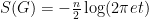
The fundamental notions of calculus, namely differentiation and integration, are often viewed as being the quintessential concepts in mathematical analysis, as their standard definitions involve the concept of a limit. However, it is possible to capture most of the essence of these notions by purely algebraic means (almost completely avoiding the use of limits, Riemann sums, and similar devices), which turns out to be useful when trying to generalise these concepts to more abstract situations in which it becomes convenient to permit the underlying number systems involved to be something other than the real or complex numbers, even if this makes many standard analysis constructions unavailable. For instance, the algebraic notion of a derivation often serves as a substitute for the analytic notion of a derivative in such cases, by abstracting out the key algebraic properties of differentiation, namely linearity and the Leibniz rule (also known as the product rule).
Abstract algebraic analogues of integration are less well known, but can still be developed. To motivate such an abstraction, consider the integration functional 


where the integration on the right is the usual Lebesgue integral (or improper Riemann integral) from analysis. This functional obeys two obvious algebraic properties. Firstly, it is linear over 

for all 

for all 


This is not quite true as stated (one can modify the proof of the Hahn-Banach theorem, after first applying a Fourier transform, to create pathological translation-invariant linear functionals on

for all 


Next, note that any Schwartz function of integral zero has an antiderivative which is also Schwartz, and so
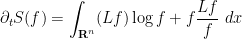
Motivated by the above discussion, we can define the notion of an abstract integration functional 


Once we have performed this abstraction, we can now present analogues of classical integration which bear very little analytic resemblance to the classical concept, but which still have much of the algebraic structure of integration. Consider for instance the situation in which we keep the complex range 


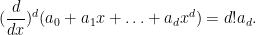
Clearly, every polynomial of degree at most 

for some constant

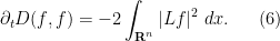
for any polynomial
In particular, we see, in contrast to the usual Lebesgue integral, the integration functional (6) can be localised to an arbitrary location: one only needs to know the germ of the polynomial 
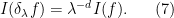
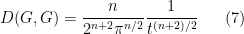
The reversal of the relationship between integration and differentiation is also reflected in the fact that the abstract integration operation on polynomials interacts with the scaling operation 


for Schwartz functions 
In contrast, the abstract integration operation defined in (6) obeys the opposite scaling law
Remark 1 One way to interpret what is going on is to view the integration operation (6) as a renormalised version of integration. A polynomial
is, in general, not absolutely integrable, and the partial integrals
diverge as
. But if one renormalises these integrals by the factor
, then one recovers convergence,
thus giving an interpretation of (6) as a renormalised classical integral, with the renormalisation being responsible for the unusual scaling relationship in (7). However, this interpretation is a little artificial, and it seems that it is best to view functionals such as (6) from an abstract algebraic perspective, rather than to try to force an analytic interpretation on them.

Now we return to the classical Lebesgue integral
As noted earlier, this integration functional has a translation invariance associated to translations along the real line 


whenever 

where 


Of course, the functional

However, thanks to contour shifting, we now also have translation invariance with respect to complex translation:

where of course we continue to define the translation operator 
for any 


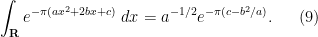
when 


using the branch of 


giving the usual gaussian integral formula
This is a basic illustration of the power that a large symmetry group (in this case, the complex homothety group) can bring to bear on the task of computing integrals.
One can extend this sort of analysis to higher dimensions. For any natural number 


whenever 


where 


where 


for 

whenever 

Now we turn to an integration functional suitable for computing complex gaussian integrals such as
where


of complex variables, which is jointly entire in all 


whenever 


thus 

and note that the integrand here is a Schwartz entire function on

for 


In particular, this gives an integral representation for the determinant-reciprocal 
This formula is then convenient for computing statistics such as
for random matrices 


However, if one restricts attention to classical integrals over real or complex (and in particular, commuting or bosonic) variables, it does not seem possible to easily eradicate the negative determinant factors in such calculations, which is unfortunate because many statistics of interest in random matrix theory, such as the expected Stieltjes transform

which is the Stieltjes transform of the density of states. However, it turns out (as I learned recently from Peter Sarnak and Tom Spencer) that it is possible to cancel out these negative determinant factors by balancing the bosonic gaussian integrals with an equal number of fermionic gaussian integrals, in which one integrates over a family of anticommuting variables. These fermionic integrals are closer in spirit to the polynomial integral (6) than to Lebesgue type integrals, and in particular obey a scaling law which is inverse to the Lebesgue scaling (in particular, a linear change of fermionic variables 

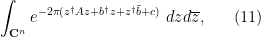
Abstract integrals of the flavour of (6) arose in quantum field theory, when physicists sought to formally compute integrals of the form

where 


In this post I would like to set out some of the basic algebraic formalism of Berezin integration, particularly with regards to integration of gaussian-type expressions, and then show how this formalism can be used to perform computations involving GUE (for instance, one can compute the density of states of GUE by this machinery without recourse to the theory of orthogonal polynomials). The use of supersymmetric gaussian integrals to analyse ensembles such as GUE appears in the work of Efetov (and was also proposed in the slightly earlier works of Parisi-Sourlas and McKane, with a related approach also appearing in the work of Wegner); the material here is adapted from this survey of Mirlin, as well as the later papers of Disertori-Pinson-Spencer and of Disertori.
Consider the free Schrödinger equation in
where 


for 


An analogous symmetry exists for the free wave equation in 
where 


also solves (3).
There are also some direct links between the Schrödinger equation in 

solves (3). More generally, for any non-zero scaling parameter 

solves (3).
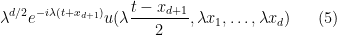
As an “extra challenge” posed in an exercise in one of my books (Exercise 2.28, to be precise), I asked the reader to use the embeddings 


Let 

where 


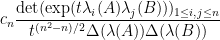
when the eigenvalues of 

and 

There are at least two standard ways to prove this formula in the literature. One way is by applying the Duistermaat-Heckman theorem to the pushforward of Liouville measure on the coadjoint orbit 

The Harish-Chandra-Itzykson-Zuber formula can be extended to other compact Lie groups than 
[These are notes intended mostly for myself, as these topics are useful in random matrix theory, but may be of interest to some readers also. -T.]
One of the most fundamental partial differential equations in mathematics is the heat equation
where 


In probability theory, this equation takes on particular significance when
for all 
where 

A model example of a solution to the heat equation to keep in mind is that of the fundamental solution

defined for any 


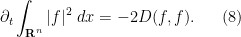
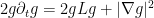
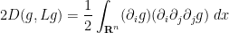
The heat equation can also be viewed as the gradient flow for the Dirichlet form
since one has the integration by parts identity

for all smooth, rapidly decreasing 


For instance, for the fundamental solution (3), one can verify for any time
(assuming I have not made a mistake in the calculation). In a similar spirit we have
Since 


Since 

for any function
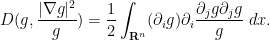
There are other quantities relating to
Thus, for instance, if 


A short formal computation shows (if one assumes for simplicity that


where 

In particular, the entropy is decreasing, which corresponds well to one’s intuition that the heat equation (or Brownian motion) should serve to spread out a probability distribution over time.
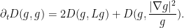
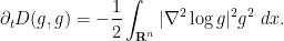
Actually, one can say more: the rate of decrease 

valid for for any smooth function 
and thus (again assuming that 

We thus have
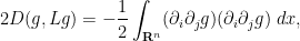
It is now convenient to compute using the Einstein summation convention to hide the summation over indices 
and
By integration by parts and interchanging partial derivatives, we may write the first integral as
and from the quotient and product rules, we may write the second integral as

Gathering terms, completing the square, and making the summations explicit again, we see that

and so in particular 
The above identity can also be written as
Exercise 1 Give an alternate proof of the above identity by writing
,
and deriving the equation
for
It was observed in a well known paper of Bakry and Emery that the above monotonicity properties hold for a much larger class of heat flow-type equations, and lead to a number of important relations between energy and entropy, such as the log-Sobolev inequality of Gross and of Federbush, and the hypercontractivity inequality of Nelson; we will discuss one such family of generalisations (or more precisely, variants) below the fold.
Emmanuel Breuillard, Ben Green, and I have just uploaded to the arXiv our survey “Small doubling in groups“, for the proceedings of the upcoming Erdos Centennial. This is a short survey of the known results on classifying finite subsets 


In the classical case when 

Freiman’s original theorem was extended to more general abelian groups in a sequence of papers culminating in the paper of Green and Ruzsa that handled arbitrary abelian groups. As such groups now contain non-trivial finite subgroups, the conclusion of the theorem must be modified by allowing for “coset progressions” 

The proof methods in these abelian results were Fourier-analytic in nature (except in the cases of sets of very small doubling, in which more combinatorial approaches can be applied, and there were also some geometric or combinatorial methods that gave some weaker structural results). As such, it was a challenge to extend these results to nonabelian groups, although for various important special types of ambient group
This survey is too short to discuss in much detail the proof techniques used in these results (although the abelian case is discussed in this book of mine with Vu, and the nonabelian case discussed in this more recent book of mine), but instead focuses on the statements of the various known results, as well as some remaining open questions in the subject (in particular, there is substantial work left to be done in making the estimates more quantitative, particularly in the nonabelian setting).

Recent Comments