More Mahler lectures

I am posting here four more of my Mahler lectures, each of which is based on earlier talks of mine:

• Compressed sensing.  This is an updated and reformatted version of my ANZIAM talk on this topic.
• Discrete random matrices.  This talk is a survey on recent developments on the universality phenomenon in random matrices, including work of myself and Van Vu.  It covers similar material to my Netanyahu lecture, which has not previously appeared in electronic form.
• Recent progress in additive prime number theory.  This is an updated and reformatted version of my AMS lecture on this topic.
• Recent progress on the Kakeya conjecture.  This is an updated and reformatted version of my Fefferman conference lecture.

As always, comments, corrections, and other feedback are welcome.

A remark on partial sums involving the Möbius function

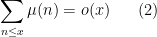
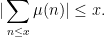
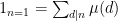
I’ve just uploaded to the arXiv the paper A remark on partial sums involving the Möbius function, submitted to Bull. Aust. Math. Soc..

The Möbius function is defined to equal when is the product of distinct primes, and equal to zero otherwise; it is closely connected to the distribution of the primes. In 1906, Landau observed that one could show using purely elementary means that the prime number theorem

(where denotes a quantity that goes to zero as ) was logically equivalent to the partial sum estimates

and

we give a sketch of the proof of these equivalences below the fold.

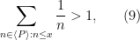
On the other hand, these three inequalities are all easy to prove if the terms are replaced by their counterparts. For instance, by observing that the binomial coefficient is bounded by on the one hand (by Pascal’s triangle or the binomial theorem), and is divisible by every prime between and on the other hand, we conclude that

from which it is not difficult to show that

Also, since , we clearly have

Finally, one can also show that

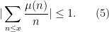
Indeed, assuming without loss of generality that is a positive integer, and summing the inversion formula over all one sees that

and the claim follows by bounding by .

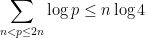
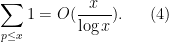
In this paper I extend these observations to more general multiplicative subsemigroups of the natural numbers. More precisely, if is any set of primes (finite or infinite), I show that

and that

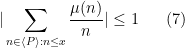
where is the multiplicative semigroup generated by , i.e. the set of natural numbers whose prime factors lie in .

Actually the methods are completely elementary (the paper is just six pages long), and I can give the proof of (7) in full here. Again we may take to be a positive integer. Clearly we may assume that

as the claim is trivial otherwise.

If denotes the primes that are not in , then Möbius inversion gives us

Summing this for gives

We can bound 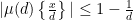and so

The claim now follows from (9), since and overlap only at .

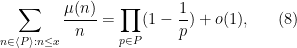
As special cases of (7) we see that

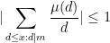
and

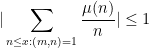
for all . Since , we also have

One might hope that these inequalities (which gain a factor of over the trivial bound) might be useful when performing effective sieve theory, or effective estimates on various sums involving the primes or arithmetic functions.

This inequality (7) is so simple to state and prove that I must think that it was known to, say, Landau or Chebyshev, but I can’t find any reference to it in the literature. [Update, Sep 4: I have learned that similar results have been obtained in a paper by Granville and Soundararajan, and have updated the paper appropriately.] The proof of (8) is a simple variant of that used to prove (7) but I will not detail it here.

Curiously, this is one place in number theory where the elementary methods seem superior to the analytic ones; there is a zeta function associated to this problem, but it need not have a meromorphic continuation beyond the region , and it turns out to be remarkably difficult to use this function to establish the above results. (I do have a proof of this form, which I in fact found before I stumbled on the elementary proof, but it is far longer and messier.)

Mathematical research and the internet

I’ll be in Australia for the next month or so, giving my share of the Clay-Mahler lectures at various institutions in the country.  My first lecture is next Monday at Melbourne University, entitled “Mathematical research and the internet“.  This public lecture discusses how various internet technologies (such as blogging) are beginning to transform the way mathematicians do research.

In the spirit of that article, I have decided to upload an advance copy of the talk here, and would welcome any comments or feedback (I still have a little bit of time to revise the article).   [NB: the PDF file is about 5MB in size; the original Powerpoint presentation was 10MB!]

[Update, August 31: the talk has been updated in view of feedback from this blog and elsewhere.  For comparison, the older version of the talk can be found here.]

[Update, Sep 4: Video of the talk and other information is available here.]

Determinantal processes

Given a set , a (simple) point process is a random subset of . (A non-simple point process would allow multiplicity; more formally, is no longer a subset of , but is a Radon measure on , where we give the structure of a locally compact Polish space, but I do not wish to dwell on these sorts of technical issues here.) Typically, will be finite or countable, even when is uncountable. Basic examples of point processes include

• (Bernoulli point process) is an at most countable set, is a parameter, and a random set such that the events for each are jointly independent and occur with a probability of each. This process is automatically simple.
• (Discrete Poisson point process) is an at most countable space, is a measure on (i.e. an assignment of a non-negative number to each ), and is a multiset where the multiplicity of in is a Poisson random variable with intensity , and the multiplicities of as varies in are jointly independent. This process is usually not simple.
• (Continuous Poisson point process) is a locally compact Polish space with a Radon measure , and for each of finite measure, the number of points that contains inside is a Poisson random variable with intensity . Furthermore, if are disjoint sets, then the random variables are jointly independent. (The fact that Poisson processes exist at all requires a non-trivial amount of measure theory, and will not be discussed here.) This process is almost surely simple iff all points in have measure zero.
• (Spectral point processes) The spectrum of a random matrix is a point process in (or in , if the random matrix is Hermitian). If the spectrum is almost surely simple, then the point process is almost surely simple. In a similar spirit, the zeroes of a random polynomial are also a point process.

A remarkable fact is that many natural (simple) point processes are determinantal processes. Very roughly speaking, this means that there exists a positive semi-definite kernel such that, for any , the probability that all lie in the random set is proportional to the determinant . Examples of processes known to be determinantal include non-intersecting random walks, spectra of random matrix ensembles such as GUE, and zeroes of polynomials with gaussian coefficients.

I would be interested in finding a good explanation (even at the heuristic level) as to why determinantal processes are so prevalent in practice. I do have a very weak explanation, namely that determinantal processes obey a large number of rather pretty algebraic identities, and so it is plausible that any other process which has a very algebraic structure (in particular, any process involving gaussians, characteristic polynomials, etc.) would be connected in some way with determinantal processes. I’m not particularly satisfied with this explanation, but I thought I would at least describe some of these identities below to support this case. (This is partly for my own benefit, as I am trying to learn about these processes, particularly in connection with the spectral distribution of random matrices.) The material here is partly based on this survey of Hough, Krishnapur, Peres, and Virág.

The least quadratic nonresidue, and the square root barrier

A large portion of analytic number theory is concerned with the distribution of number-theoretic sets such as the primes, or quadratic residues in a certain modulus. At a local level (e.g. on a short interval ), the behaviour of these sets may be quite irregular. However, in many cases one can understand the global behaviour of such sets on very large intervals, (e.g. ), with reasonable accuracy (particularly if one assumes powerful additional conjectures, such as the Riemann hypothesis and its generalisations). For instance, in the case of the primes, we have the prime number theorem, which asserts that the number of primes in a large interval is asymptotically equal to ; in the case of quadratic residues modulo a prime , it is clear that there are exactly such residues in . With elementary arguments, one can also count statistics such as the number of pairs of consecutive quadratic residues; and with the aid of deeper tools such as the Weil sum estimates, one can count more complex patterns in these residues also (e.g. -point correlations).

One is often interested in converting this sort of “global” information on long intervals into “local” information on short intervals. If one is interested in the behaviour on a generic or average short interval, then the question is still essentially a global one, basically because one can view a long interval as an average of a long sequence of short intervals. (This does not mean that the problem is automatically easy, because not every global statistic about, say, the primes is understood. For instance, we do not know how to rigorously establish the conjectured asymptotic for the number of twin primes in a long interval , and so we do not fully understand the local distribution of the primes in a typical short interval .)

However, suppose that instead of understanding the average-case behaviour of short intervals, one wants to control the worst-case behaviour of such intervals (i.e. to establish bounds that hold for all short intervals, rather than most short intervals). Then it becomes substantially harder to convert global information to local information. In many cases one encounters a “square root barrier”, in which global information at scale (e.g. statistics on ) cannot be used to say anything non-trivial about a fixed (and possibly worst-case) short interval at scales or below. (Here we ignore factors of for simplicity.) The basic reason for this is that even randomly distributed sets in (which are basically the most uniform type of global distribution one could hope for) exhibit random fluctuations of size or so in their global statistics (as can be seen for instance from the central limit theorem). Because of this, one could take a random (or pseudorandom) subset of and delete all the elements in a short interval of length , without anything suspicious showing up on the global statistics level; the edited set still has essentially the same global statistics as the original set. On the other hand, the worst-case behaviour of this set on a short interval has been drastically altered.

One stark example of this arises when trying to control the largest gap between consecutive prime numbers in a large interval . There are convincing heuristics that suggest that this largest gap is of size (Cramér’s conjecture). But even assuming the Riemann hypothesis, the best upper bound on this gap is only of size , basically because of this square root barrier. This particular instance of the square root barrier is a significant obstruction to the current polymath project “Finding primes“.

On the other hand, in some cases one can use additional tricks to get past the square root barrier. The key point is that many number-theoretic sequences have special structure that distinguish them from being exactly like random sets. For instance, quadratic residues have the basic but fundamental property that the product of two quadratic residues is again a quadratic residue. One way to use this sort of structure to amplify bad behaviour in a single short interval into bad behaviour across many short intervals. Because of this amplification, one can sometimes get new worst-case bounds by tapping the average-case bounds.

In this post I would like to indicate a classical example of this type of amplification trick, namely Burgess’s bound on short character sums. To narrow the discussion, I would like to focus primarily on the following classical problem:

Problem 1 What are the best bounds one can place on the first quadratic non-residue in the interval for a large prime ?

(The first quadratic residue is, of course, ; the more interesting problem is the first quadratic non-residue.)

Probabilistic heuristics (presuming that each non-square integer has a 50-50 chance of being a quadratic residue) suggests that should have size , and indeed Vinogradov conjectured that for any . Using the Pólya-Vinogradov inequality, one can get the bound (and can improve it to using smoothed sums); combining this with a sieve theory argument (exploiting the multiplicative nature of quadratic residues) one can boost this to . Inserting Burgess’s amplification trick one can boost this to for any . Apart from refinements to the factor, this bound has stood for five decades as the “world record” for this problem, which is a testament to the difficulty in breaching the square root barrier.

Note: in order not to obscure the presentation with technical details, I will be using asymptotic notation in a somewhat informal manner.

Random matrices: Universality of local eigenvalue statistics up to the edge

Van Vu and I have just uploaded to the arXiv our paper “Random matrices: Universality of local eigenvalue statistics up to the edge“, submitted to Comm. Math. Phys..  This is a sequel to our previous paper, in which we studied universality of local eigenvalue statistics (such as normalised eigenvalue spacings ) for random matrices of Wigner type, i.e. Hermitian (or symmetric) random matrices in which the upper-triangular entries are independent with mean zero and variance one (for technical reasons we also have to assume an exponential decay condition on the distribution of the entries).   The results in the previous paper were almost entirely focused on the bulk region, in which the index i of the eigenvalues involved was in the range .  The main purpose of this paper is to extend the main results of the previous paper all the way up to the edge, thus allowing one to control all indices .  As an application, we obtain a variant of Soshnikov’s well-known result that the largest eigenvalue of Wigner matrices is distributed (after suitable normalisation) according to the Tracy-Widom law when the coefficients are symmetric, by assuming instead that the coefficients have vanishing third moment.

As one transitions from the bulk to the edge, the density of the eigenvalues decreases to zero (in accordance to the Wigner semicircular law), and so the average spacing between eigenvalues increases.  (For instance, the spacing between eigenvalues in the bulk is of size , but at the extreme edge it increases to .)  On the one hand, the increase in average spacing should make life easier, because one does not have to work at such a fine spatial scale in order to see the eigenvalue distribution.  On the other hand, a certain key technical step in the previous paper (in which we adapted an argument of Erdos, Schlein, and Yau to show that eigenvectors of Wigner matrices were delocalised) seemed to require eigenvalue spacings to be of size , which was the main technical obstacle to extending the preceding results from the bulk to the edge.

The main new observation in the paper is that it was not the eigenvalue spacings which were of importance to eigenvalue delocalisation, but rather the somewhat smaller interlaced eigenvalue spacings , where is a minor of .  The Cauchy interlacing law asserts that the latter is smaller than the former.  But the interesting thing is that at the edge (when i is close to n), the interlaced spacings are much smaller than the former, and in particular remain of size about (up to log factors) even though the non-interlaced spacings increase to be as large as .  This is ultimately due to a sort of “attractive force” on eigenvalues that draws them towards the origin, and counteracts the usual “eigenvalue repulsion effect”, that pushes eigenvalues away from each other.  This induces “bias” for eigenvalues to move in towards the bulk rescues the delocalization result, and the remainder of the arguments in our previous paper then continue with few changes.

Below the fold I wish to give some heuristic justification of the interlacing bias phenomenon, sketch why this is relevant for eigenvector delocalisation, and finally to recall why eigenvalue delocalisation in turn is relevant for universality.

[Update, Aug 16: sign error corrected.]

The AKS primality test

The Agrawal-Kayal-Saxena (AKS) primality test, discovered in 2002, is the first provably deterministic algorithm to determine the primality of a given number with a run time which is guaranteed to be polynomial in the number of digits, thus, given a large number , the algorithm will correctly determine whether that number is prime or not in time . (Many previous primality testing algorithms existed, but they were either probabilistic in nature, had a running time slower than polynomial, or the correctness could not be guaranteed without additional hypotheses such as GRH.)

The AKS test is of some relevance to the polymath project “Finding primes“, so I thought I would sketch the details of the test (and the proof that it works) here. (Of course, full details can be found in the original paper, which is nine pages in length and almost entirely elementary in nature.) It relies on polynomial identities that are true modulo when is prime, but cannot hold for non-prime as they would generate a large number of additional polynomial identities, eventually violating the factor theorem (which asserts that a polynomial identity of degree at most can be obeyed by at most values of the unknown).

Mathematics/Statistics blogs wiki page

In the discussion on what mathematicians need to know about blogging mentioned in the previous post, it was noted that there didn’t seem to be a single location on the internet to find out about mathematical blogs.  Actually, there is a page, but it has been relatively obscure – the Mathematics/Statistics subpage of the Academic Blogs wiki.  It does seem like a good idea to have a reasonably comprehensive page containing all the academic mathematics blogs that are out there (as well as links to other relevant sites), so I put my own maths blogroll onto the page, and encourage others to do so also (though you may wish to read the FAQ for the wiki first).

It may also be useful to organise the list into sublists, and to add more commentary on each individual blog.  (In theory, each blog is supposed to have its own sub-page, though in practice it seems that very few blogs do at present.)

What do mathematicians need to know about blogging?

John Baez has been invited to write a short opinion piece for the Notices of the AMS to report about the maths blogging phenomenon to the wider mathematical community, and in the spirit of that phenomenon, has opened up a blog post to solicit input for that piece, over at the n-Category café.  Given that the readers here are, by definition, familiar with mathematical blogging, I thought that some of you might like to visit that thread to share your own thoughts on the advantages and disadvantages of this mode of mathematical communication.

Polymath4 (“Finding Primes”) now officially active

The polymath project “Finding primes” has now officially launched at the polymath blog as Polymath4, with the opening of a fresh research thread to discuss the following problem:

Problem 1. Find a deterministic algorithm which, when given an integer k, is guaranteed to locate a prime of at least k digits, in time polynomial in k.

From the preliminary research thread, we’ve discovered some good reasons why this problem is difficult (unless one assumes some powerful conjectures in number theory or complexity theory), so we have also identified some simpler toy problems:

Problem 2. Find a deterministic algorithm which, when given an integer k, is guaranteed to locate an adjacent pair n, n+1 of square-free numbers of at least k digits, in time polynomial in k.

(Note that finding one large square-free number is easy – just multiply a lot of small primes together.  Adjacent large square-free numbers exist in abundance, but it is not obvious how to actually find one deterministically and quickly.)

Problem 3. Assume access to a factoring oracle.  Find an algorithm which, when given an integer k, is guaranteed to find a prime of at least  k digits (or an integer divisible by a prime of at least k digits) in time .

The current record time is unconditionally, or about on the Riemann hypothesis.

In the new research thread, a number of possible strategies are discussed, and will hopefully be explored soon.  In addition to this thread, there is also the wiki page for the project, and a discussion thread aimed at more casual participants.  Everyone is welcome to contribute to any of these three components of the project, as always.