
You are currently browsing the monthly archive for March 2019.
I was pleased to learn this week that the 2019 Abel Prize was awarded to Karen Uhlenbeck. Uhlenbeck laid much of the foundations of modern geometric PDE. One of the few papers I have in this area is in fact a joint paper with Gang Tian extending a famous singularity removal theorem of Uhlenbeck for four-dimensional Yang-Mills connections to higher dimensions. In both these papers, it is crucial to be able to construct “Coulomb gauges” for various connections, and there is a clever trick of Uhlenbeck for doing so, introduced in another important paper of hers, which is absolutely critical in my own paper with Tian. Nowadays it would be considered a standard technique, but it was definitely not so at the time that Uhlenbeck introduced it.
Suppose one has a smooth connection 


![\displaystyle F(A)_{\alpha \beta} = \partial_\alpha A_\beta - \partial_\beta A_\alpha + [A_\alpha,A_\beta]. \ \ \ \ \ (1)](https://s0.wp.com/latex.php?latex=%5Cdisplaystyle+F%28A%29_%7B%5Calpha+%5Cbeta%7D+%3D+%5Cpartial_%5Calpha+A_%5Cbeta+-+%5Cpartial_%5Cbeta+A_%5Calpha+%2B+%5BA_%5Calpha%2CA_%5Cbeta%5D.+%5C+%5C+%5C+%5C+%5C+%281%29&bg=ffffff&fg=000000&s=0&c=20201002)
It is natural to place the curvature in a scale-invariant space such as 
There is a basic obstruction provided by gauge invariance. For any smooth gauge 

and then a brief calculation shows that the curvature is conjugated to
This gauge symmetry does not affect the 
However, one can hope to overcome this problem by gauge fixing: perhaps if 

To make the problem elliptic, one can try to impose the Coulomb gauge condition

(also known as the Lorenz gauge or Hodge gauge in various papers), together with a natural boundary condition on 
![\displaystyle \partial^\alpha F(A)_{\alpha \beta} = \Delta A_\beta + \partial^\alpha [A_\alpha,A_\beta] \ \ \ \ \ (3)](https://s0.wp.com/latex.php?latex=%5Cdisplaystyle+%5Cpartial%5E%5Calpha+F%28A%29_%7B%5Calpha+%5Cbeta%7D+%3D+%5CDelta+A_%5Cbeta+%2B+%5Cpartial%5E%5Calpha+%5BA_%5Calpha%2CA_%5Cbeta%5D+%5C+%5C+%5C+%5C+%5C+%283%29&bg=ffffff&fg=000000&s=0&c=20201002)
and if one could somehow ignore the nonlinear term ![{\partial^\alpha [A_\alpha,A_\beta]}](https://s0.wp.com/latex.php?latex=%7B%5Cpartial%5E%5Calpha+%5BA_%5Calpha%2CA_%5Cbeta%5D%7D&bg=ffffff&fg=000000&s=0&c=20201002)
The problem is then how to handle the nonlinear term. If we already knew that
Uhlenbeck’s clever way out of this circularity is a textbook example of what is now known as a “continuity” argument. Instead of trying to work just with the original connection 


![{t \in [0,1]}](https://s0.wp.com/latex.php?latex=%7Bt+%5Cin+%5B0%2C1%5D%7D&bg=ffffff&fg=000000&s=0&c=20201002)


![{t' \in [0,1]}](https://s0.wp.com/latex.php?latex=%7Bt%27+%5Cin+%5B0%2C1%5D%7D&bg=ffffff&fg=000000&s=0&c=20201002)


![{[0,1]}](https://s0.wp.com/latex.php?latex=%7B%5B0%2C1%5D%7D&bg=ffffff&fg=000000&s=0&c=20201002)
One of the lessons I drew from this example is to not be deterred (especially in PDE) by an argument seeming to be circular; if the argument is still sufficiently “nontrivial” in nature, it can often be modified into a usefully non-circular argument that achieves what one wants (possibly under an additional qualitative hypothesis, such as a continuity or smoothness hypothesis).
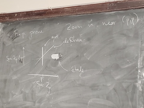
Last week, we had Peter Scholze give an interesting distinguished lecture series here at UCLA on “Prismatic Cohomology”, which is a new type of cohomology theory worked out by Scholze and Bhargav Bhatt. (Video of the talks will be available shortly; for now we have some notes taken by two note–takers in the audience on that web page.) My understanding of this (speaking as someone that is rather far removed from this area) is that it is progress towards the “motivic” dream of being able to define cohomology 


- Singular cohomology, which roughly speaking works when the domain ring
or
, but can allow for arbitrary coefficients
- de Rham cohomology, which roughly speaking works as long as the coefficient ring
-adic cohomology, which is a remarkably powerful application of étale cohomology, but only works well when the coefficient ring
is localised around a prime
of the domain ring
- Crystalline cohomology, in which the domain ring is a field
of some finite characteristic
There are various relationships between the cohomology theories, for instance de Rham cohomology coincides with singular cohomology for smooth varieties in the limiting case 
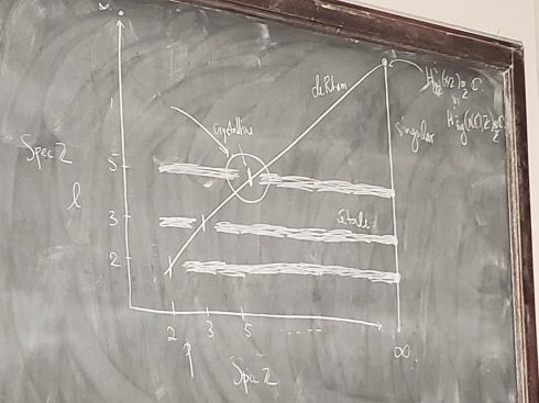
The new prismatic cohomology of Bhatt and Scholze unifies many of these cohomologies in the “neighbourhood” of the point 


To define prismatic cohomology rings 


(And yes, Peter confirmed that he and Bhargav were inspired by the Dark Side of the Moon album cover in selecting the terminology.)
There was an abstract definition of prismatic cohomology (as being the essentially unique cohomology arising from prisms that obeyed certain natural axioms), but there was also a more concrete way to view them in terms of coordinates, as a “


prismatic cohomology in coordinates can be computed using a “
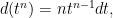
![\displaystyle d_q (t^n) = [n]_q t^{n-1} d_q t](https://s0.wp.com/latex.php?latex=%5Cdisplaystyle+d_q+%28t%5En%29+%3D+%5Bn%5D_q+t%5E%7Bn-1%7D+d_q+t&bg=ffffff&fg=000000&s=0&c=20201002)
where
![\displaystyle [n]_q = \frac{q^n-1}{q-1} = 1 + q + \dots + q^{n-1}](https://s0.wp.com/latex.php?latex=%5Cdisplaystyle+%5Bn%5D_q+%3D+%5Cfrac%7Bq%5En-1%7D%7Bq-1%7D+%3D+1+%2B+q+%2B+%5Cdots+%2B+q%5E%7Bn-1%7D&bg=ffffff&fg=000000&s=0&c=20201002)
is the “


Recent Comments