Random matrices: tail bounds for gaps between eigenvalues

Hoi Nguyen, Van Vu, and myself have just uploaded to the arXiv our paper “Random matrices: tail bounds for gaps between eigenvalues“. This is a followup paper to my recent paper with Van in which we showed that random matrices of Wigner type (such as the adjacency matrix of an Erdös-Renyi graph) asymptotically almost surely had simple spectrum. In the current paper, we push the method further to show that the eigenvalues are not only distinct, but are (with high probability) separated from each other by some negative power of . This follows the now standard technique of replacing any appearance of discrete Littlewood-Offord theory (a key ingredient in our previous paper) with its continuous analogue (inverse theorems for small ball probability). For general Wigner-type matrices (in which the matrix entries are not normalised to have mean zero), we can use the inverse Littlewood-Offord theorem of Nguyen and Vu to obtain (under mild conditions on ) a result of the form

for any and , if is sufficiently large depending on (in a linear fashion), and is sufficiently large depending on . The point here is that can be made arbitrarily large, and also that no continuity or smoothness hypothesis is made on the distribution of the entries. (In the continuous case, one can use the machinery of Wegner estimates to obtain results of this type, as was done in a paper of Erdös, Schlein, and Yau.)

In the mean zero case, it becomes more efficient to use an inverse Littlewood-Offord theorem of Rudelson and Vershynin to obtain (with the normalisation that the entries of have unit variance, so that the eigenvalues of are with high probability), giving the bound

for (one also has good results of this type for smaller values of ). This is only optimal in the regime ; we expect to establish some eigenvalue repulsion, improving the RHS to for real matrices and for complex matrices, but this appears to be a more difficult task (possibly requiring some quadratic inverse Littlewood-Offord theory, rather than just linear inverse Littlewood-Offord theory). However, we can get some repulsion if one works with larger gaps, getting a result roughly of the form

for any fixed and some absolute constant (which we can asymptotically make to be for large , though it ought to be as large as ), by using a higher-dimensional version of the Rudelson-Vershynin inverse Littlewood-Offord theorem.

In the case of Erdös-Renyi graphs, we don’t have mean zero and the Rudelson-Vershynin Littlewood-Offord theorem isn’t quite applicable, but by working carefully through the approach based on the Nguyen-Vu theorem we can almost recover (1), except for a loss of on the RHS.

As a sample applications of the eigenvalue separation results, we can now obtain some information about eigenvectors; for instance, we can show that the components of the eigenvectors all have magnitude at least for some with high probability. (Eigenvectors become much more stable, and able to be studied in isolation, once their associated eigenvalue is well separated from the other eigenvalues; see this previous blog post for more discussion.)

Random matrices have simple spectrum

Van Vu and I have just uploaded to the arXiv our paper “Random matrices have simple spectrum“. Recall that an Hermitian matrix is said to have simple eigenvalues if all of its eigenvalues are distinct. This is a very typical property of matrices to have: for instance, as discussed in this previous post, in the space of all Hermitian matrices, the space of matrices without all eigenvalues simple has codimension three, and for real symmetric cases this space has codimension two. In particular, given any random matrix ensemble of Hermitian or real symmetric matrices with an absolutely continuous distribution, we conclude that random matrices drawn from this ensemble will almost surely have simple eigenvalues.

For discrete random matrix ensembles, though, the above argument breaks down, even though general universality heuristics predict that the statistics of discrete ensembles should behave similarly to those of continuous ensembles. A model case here is the adjacency matrix of an Erdös-Rényi graph – a graph on vertices in which any pair of vertices has an independent probability of being in the graph. For the purposes of this paper one should view as fixed, e.g. , while is an asymptotic parameter going to infinity. In this context, our main result is the following (answering a question of Babai):

Theorem 1 With probability , has simple eigenvalues.

Our argument works for more general Wigner-type matrix ensembles, but for sake of illustration we will stick with the Erdös-Renyi case. Previous work on local universality for such matrix models (e.g. the work of Erdos, Knowles, Yau, and Yin) was able to show that any individual eigenvalue gap 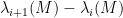did not vanish with probability (in fact for some absolute constant ), but because there are different gaps that one has to simultaneously ensure to be non-zero, this did not give Theorem 1 as one is forced to apply the union bound.

Our argument in fact gives simplicity of the spectrum with probability for any fixed ; in a subsequent paper we also show that it gives a quantitative lower bound on the eigenvalue gaps (analogous to how many results on the singularity probability of random matrices can be upgraded to a bound on the least singular value).

The basic idea of argument can be sketched as follows. Suppose that has a repeated eigenvalue . We split

for a random minor and a random sign vector ; crucially, and are independent. If has a repeated eigenvalue , then by the Cauchy interlacing law, also has an eigenvalue . We now write down the eigenvector equation for at :

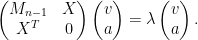
Extracting the top coefficients, we obtain

If we let be the -eigenvector of , then by taking inner products with we conclude that

we typically expect to be non-zero, in which case we arrive at

In other words, in order for to have a repeated eigenvalue, the top right column of has to be orthogonal to an eigenvector of the minor . Note that and are going to be independent (once we specify which eigenvector of to take as ). On the other hand, thanks to inverse Littlewood-Offord theory (specifically, we use an inverse Littlewood-Offord theorem of Nguyen and Vu), we know that the vector is unlikely to be orthogonal to any given vector independent of , unless the coefficients of are extremely special (specifically, that most of them lie in a generalised arithmetic progression). The main remaining difficulty is then to show that eigenvectors of a random matrix are typically not of this special form, and this relies on a conditioning argument originally used by Komlós to bound the singularity probability of a random sign matrix. (Basically, if an eigenvector has this special form, then one can use a fraction of the rows and columns of the random matrix to determine the eigenvector completely, while still preserving enough randomness in the remaining portion of the matrix so that this vector will in fact not be an eigenvector with high probability.)

The Collatz conjecture, Littlewood-Offord theory, and powers of 2 and 3

One of the most notorious problems in elementary mathematics that remains unsolved is the Collatz conjecture, concerning the function defined by setting when is odd, and when is even. (Here, is understood to be the positive natural numbers .)

Conjecture 1 (Collatz conjecture) For any given natural number , the orbit passes through (i.e. for some ).

Open questions with this level of notoriety can lead to what Richard Lipton calls “mathematical diseases” (and what I termed an unhealthy amount of obsession on a single famous problem). (See also this xkcd comic regarding the Collatz conjecture.) As such, most practicing mathematicians tend to spend the majority of their time on more productive research areas that are only just beyond the range of current techniques. Nevertheless, it can still be diverting to spend a day or two each year on these sorts of questions, before returning to other matters; so I recently had a go at the problem. Needless to say, I didn’t solve the problem, but I have a better appreciation of why the conjecture is (a) plausible, and (b) unlikely be proven by current technology, and I thought I would share what I had found out here on this blog.

Let me begin with some very well known facts. If is odd, then is even, and so . Because of this, one could replace by the function , defined by when is odd, and when is even, and obtain an equivalent conjecture. Now we see that if one chooses “at random”, in the sense that it is odd with probability and even with probability , then increases by a factor of roughly half the time, and decreases it by a factor of half the time. Furthermore, if is uniformly distributed modulo , one easily verifies that is uniformly distributed modulo , and so should be roughly times as large as half the time, and roughly times as large as the other half of the time. Continuing this at a heuristic level, we expect generically that half the time, and the other half of the time. The logarithm of this orbit can then be modeled heuristically by a random walk with steps and occuring with equal probability. The expectation

is negative, and so (by the classic gambler’s ruin) we expect the orbit to decrease over the long term. This can be viewed as heuristic justification of the Collatz conjecture, at least in the “average case” scenario in which is chosen uniform at random (e.g. in some large interval ). (It also suggests that if one modifies the problem, e.g. by replacing to , then one can obtain orbits that tend to increase over time, and indeed numerically for this variant one sees orbits that appear to escape to infinity.) Unfortunately, one can only rigorously keep the orbit uniformly distributed modulo for time about or so; after that, the system is too complicated for naive methods to control at anything other than a heuristic level.

Remark 1 One can obtain a rigorous analogue of the above arguments by extending from the integers to the -adics . This compact abelian group comes with a Haar probability measure, and one can verify that this measure is invariant with respect to ; with a bit more effort one can verify that it is ergodic. This suggests the introduction of ergodic theory methods. For instance, using the pointwise ergodic theorem, we see that if is a random -adic integer, then almost surely the orbit will be even half the time and odd half the time asymptotically, thus supporting the above heuristics. Unfortunately, this does not directly tell us much about the dynamics on , as this is a measure zero subset of . More generally, unless a dynamical system is somehow “polynomial”, “nilpotent”, or “unipotent” in nature, the current state of ergodic theory is usually only able to say something meaningful about generic orbits, but not about all orbits. For instance, the very simple system on the unit circle is well understood from ergodic theory (in particular, almost all orbits will be uniformly distributed), but the orbit of a specific point, e.g. , is still nearly impossible to understand (this particular problem being equivalent to the notorious unsolved question of whether the digits of are uniformly distributed).

The above heuristic argument only suggests decreasing orbits for almost all (though even this remains unproven, the state of the art is that the number of in that eventually go to is , a result of Krasikov and Lagarias). It leaves open the possibility of some very rare exceptional for which the orbit goes to infinity, or gets trapped in a periodic loop. Since the only loop that lies in is (for ) or (for ), we thus may isolate a weaker consequence of the Collatz conjecture:

Conjecture 2 (Weak Collatz conjecture) Suppose that is a natural number such that for some . Then is equal to , , or .

Of course, we may replace with (and delete ““) and obtain an equivalent conjecture.

This weaker version of the Collatz conjecture is also unproven. However, it was observed by Bohm and Sontacchi that this weak conjecture is equivalent to a divisibility problem involving powers of and :

Conjecture 3 (Reformulated weak Collatz conjecture) There does not exist and integers

such that is a positive integer that is a proper divisor of

i.e.

 

for some natural number .

Proposition 4 Conjecture 2 and Conjecture 3 are equivalent.

Proof: To see this, it is convenient to reformulate Conjecture 2 slightly. Define an equivalence relation on by declaring if for some integer , thus giving rise to the quotient space of equivalence classes (which can be placed, if one wishes, in one-to-one correspondence with the odd natural numbers). We can then define a function by declaring

 

for any , where is the largest power of that divides . It is easy to see that is well-defined (it is essentially the Syracuse function, after identifying with the odd natural numbers), and that periodic orbits of correspond to periodic orbits of or . Thus, Conjecture 2 is equivalent to the conjecture that is the only periodic orbit of .

Now suppose that Conjecture 2 failed, thus there exists such that for some . Without loss of generality we may take to be odd, then . It is easy to see that is the only fixed point of , and so . An easy induction using (2) shows that

where, for each , is the largest power of that divides

 

In particular, as is odd, . Using the recursion

 

we see from induction that divides , and thus :

Since , we have

for some integer . Since is divisible by , and is odd, we conclude ; if we rearrange the above equation as (1), then we obtain a counterexample to Conjecture 3.

Conversely, suppose that Conjecture 3 failed. Then we have , integers

and a natural number such that (1) holds. As , we see that the right-hand side of (1) is odd, so is odd also. If we then introduce the natural numbers by the formula (3), then an easy induction using (4) shows that

 

with the periodic convention for . As the are increasing in (even for ), we see that is the largest power of that divides the right-hand side of (5); as is odd, we conclude that is also the largest power of that divides . We conclude that

and thus is a periodic orbit of . Since is an odd number larger than , this contradicts Conjecture 3.

Call a counterexample a tuple that contradicts Conjecture 3, i.e. an integer and an increasing set of integers

such that (1) holds for some . We record a simple bound on such counterexamples, due to Terras and to Garner :

Lemma 5 (Exponent bounds) Let , and suppose that the Collatz conjecture is true for all . Let be a counterexample. Then

Proof: The first bound is immediate from the positivity of . To prove the second bound, observe from the proof of Proposition 4 that the counterexample will generate a counterexample to Conjecture 2, i.e. a non-trivial periodic orbit . As the conjecture is true for all , all terms in this orbit must be at least . An inspection of the proof of Proposition 4 reveals that this orbit consists of steps of the form , and steps of the form . As all terms are at least , the former steps can increase magnitude by a multiplicative factor of at most . As the orbit returns to where it started, we conclude that

whence the claim.

The Collatz conjecture has already been verified for many values of (up to at least , according to this web site). Inserting this into the above lemma, one can get lower bounds on . For instance, by methods such as this, it is known that any non-trivial periodic orbit has length at least , as shown in Garner’s paper (and this bound, which uses the much smaller value that was available in 1981, can surely be improved using the most recent computational bounds).

Now we can perform a heuristic count on the number of counterexamples. If we fix and , then , and from basic combinatorics we see that there are different ways to choose the remaining integers

to form a potential counterexample . As a crude heuristic, one expects that for a “random” such choice of integers, the expression (1) has a probability of holding for some integer . (Note that is not divisible by or , and so one does not expect the special structure of the right-hand side of (1) with respect to those moduli to be relevant. There will be some choices of where the right-hand side in (1) is too small to be divisible by , but using the estimates in Lemma 5, one expects this to occur very infrequently.) Thus, the total expected number of solutions for this choice of is

The heuristic number of solutions overall is then expected to be

 

where, in view of Lemma 5, one should restrict the double summation to the heuristic regime , with the approximation here accurate to many decimal places.

We need a lower bound on . Here, we will use Baker’s theorem (as discussed in this previous post), which among other things gives the lower bound

 

for some absolute constant . Meanwhile, Stirling’s formula (as discussed in this previous post) combined with the approximation gives

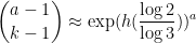
where is the entropy function

A brief computation shows that

and so (ignoring all subexponential terms)

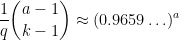
which makes the series (6) convergent. (Actually, one does not need the full strength of Lemma 5 here; anything that kept well away from would suffice. In particular, one does not need an enormous value of ; even (say) would be more than sufficient to obtain the heuristic that there are finitely many counterexamples.) Heuristically applying the Borel-Cantelli lemma, we thus expect that there are only a finite number of counterexamples to the weak Collatz conjecture (and inserting a bound such as , one in fact expects it to be extremely likely that there are no counterexamples at all).

This, of course, is far short of any rigorous proof of Conjecture 2. In order to make rigorous progress on this conjecture, it seems that one would need to somehow exploit the structural properties of numbers of the form

 

In some very special cases, this can be done. For instance, suppose that one had with at most one exception (this is essentially what is called a -cycle by Steiner). Then (8) simplifies via the geometric series formula to a combination of just a bounded number of powers of and , rather than an unbounded number. In that case, one can start using tools from transcendence theory such as Baker’s theorem to obtain good results; for instance, in the above-referenced paper of Steiner, it was shown that -cycles cannot actually occur, and similar methods have been used to show that -cycles (in which there are at most exceptions to ) do not occur for any , as was shown by Simons and de Weger. However, for general increasing tuples of integers , there is no such representation by bounded numbers of powers, and it does not seem that methods from transcendence theory will be sufficient to control the expressions (8) to the extent that one can understand their divisibility properties by quantities such as .

Amusingly, there is a slight connection to Littlewood-Offord theory in additive combinatorics – the study of the random sums

generated by some elements of an additive group , or equivalently, the vertices of an -dimensional parallelepiped inside . Here, the relevant group is . The point is that if one fixes and (and hence ), and lets vary inside the simplex

then the set of all sums of the form (8) (viewed as an element of ) contains many large parallelepipeds. (Note, incidentally, that once one fixes , all the sums of the form (8) are distinct; because given (8) and , one can read off as the largest power of that divides (8), and then subtracting off one can then read off , and so forth.) This is because the simplex contains many large cubes. Indeed, if one picks a typical element of , then one expects (thanks to Lemma 5) that there there will be indices such that for , which allows one to adjust each of the independently by if desired and still remain inside . This gives a cube in of dimension , which then induces a parallelepiped of the same dimension in . A short computation shows that the generators of this parallelepiped consist of products of a power of and a power of , and in particular will be coprime to .

If the weak Collatz conjecture is true, then the set must avoid the residue class in . Let us suppose temporarily that we did not know about Baker’s theorem (and the associated bound (7)), so that could potentially be quite small. Then we would have a large parallelepiped inside a small cyclic group that did not cover all of , which would not be possible for small enough. Indeed, an easy induction shows that a -dimensional parallelepiped in , with all generators coprime to , has cardinality at least . This argument already shows the lower bound . In other words, we have

Proposition 6 Suppose the weak Collatz conjecture is true. Then for any natural numbers with , one has .

This bound is very weak when compared against the unconditional bound (7). However, I know of no way to get a nontrivial separation property between powers of and powers of other than via transcendence theory methods. Thus, this result strongly suggests that any proof of the Collatz conjecture must either use existing results in transcendence theory, or else must contribute a new method to give non-trivial results in transcendence theory. (This already rules out a lot of possible approaches to solve the Collatz conjecture.)

By using more sophisticated tools in additive combinatorics, one can improve the above proposition (though it is still well short of the transcendence theory bound (7)):

Proposition 7 Suppose the weak Collatz conjecture is true. Then for any natural numbers with , one has for some absolute constant .

Proof: (Informal sketch only) Suppose not, then we can find with of size . We form the set as before, which contains parallelepipeds in of large dimension that avoid . We can count the number of times occurs in one of these parallelepipeds by a standard Fourier-analytic computation involving Riesz products (see Chapter 7 of my book with Van Vu, or this recent preprint of Maples). Using this Fourier representation, the fact that this parallelepiped avoids (and the fact that ) forces the generators to be concentrated in a Bohr set, in that one can find a non-zero frequency such that of the generators lie in the set . However, one can choose the generators to essentially have the structure of a (generalised) geometric progression (up to scaling, it resembles something like for ranging over a generalised arithmetic progression, and a fixed irrational), and one can show that such progressions cannot be concentrated in Bohr sets (this is similar in spirit to the exponential sum estimates of Bourgain on approximate multiplicative subgroups of , though one can use more elementary methods here due to the very strong nature of the Bohr set concentration (being of the “ concentration” variety rather than the “ concentration”).). This furnishes the required contradiction.

Thus we see that any proposed proof of the Collatz conjecture must either use transcendence theory, or introduce new techniques that are powerful enough to create exponential separation between powers of and powers of .

Unfortunately, once one uses the transcendence theory bound (7), the size of the cyclic group becomes larger than the volume of any cube in , and Littlewood-Offord techniques are no longer of much use (they can be used to show that is highly equidistributed in , but this does not directly give any way to prevent from containing ).

One possible toy model problem for the (weak) Collatz conjecture is a conjecture of Erdos asserting that for , the base representation of contains at least one . (See this paper of Lagarias for some work on this conjecture and on related problems.) To put it another way, the conjecture asserts that there are no integer solutions to

with and . (When , of course, one has .) In this form we see a resemblance to Conjecture 3, but it looks like a simpler problem to attack (though one which is still a fair distance beyond what one can do with current technology). Note that one has a similar heuristic support for this conjecture as one does for Proposition 3; a number of magnitude has about base digits, so the heuristic probability that none of these digits are equal to is , which is absolutely summable.

254A, Notes 7: The least singular value

Now we turn attention to another important spectral statistic, the least singular value of an matrix (or, more generally, the least non-trivial singular value of a matrix with ). This quantity controls the invertibility of . Indeed, is invertible precisely when is non-zero, and the operator norm of is given by . This quantity is also related to the condition number of , which is of importance in numerical linear algebra. As we shall see in the next set of notes, the least singular value of (and more generally, of the shifts for complex ) will be of importance in rigorously establishing the circular law for iid random matrices , as it plays a key role in computing the Stieltjes transform of such matrices, which as we have already seen is a powerful tool in understanding the spectra of random matrices.

The least singular value

which sits at the “hard edge” of the spectrum, bears a superficial similarity to the operator norm

at the “soft edge” of the spectrum, that was discussed back in Notes 3, so one may at first think that the methods that were effective in controlling the latter, namely the epsilon-net argument and the moment method, would also work to control the former. The epsilon-net method does indeed have some effectiveness when dealing with rectangular matrices (in which the spectrum stays well away from zero), but the situation becomes more delicate for square matrices; it can control some “low entropy” portions of the infimum that arise from “structured” or “compressible” choices of , but are not able to control the “generic” or “incompressible” choices of , for which new arguments will be needed. As for the moment method, this can give the coarse order of magnitude (for instance, for rectangular matrices with for , it gives an upper bound of for the singular value with high probability, thanks to the Marchenko-Pastur law), but again this method begins to break down for square matrices, although one can make some partial headway by considering negative moments such as , though these are more difficult to compute than positive moments .

So one needs to supplement these existing methods with additional tools. It turns out that the key issue is to understand the distance between one of the rows of the matrix , and the hyperplane spanned by the other rows. The reason for this is as follows. First suppose that , so that is non-invertible, and there is a linear dependence between the rows . Thus, one of the will lie in the hyperplane spanned by the other rows, and so one of the distances mentioned above will vanish; in fact, one expects many of the distances to vanish. Conversely, whenever one of these distances vanishes, one has a linear dependence, and so .

More generally, if the least singular value is small, one generically expects many of these distances to be small also, and conversely. Thus, control of the least singular value is morally equivalent to control of the distance between a row and the hyperplane spanned by the other rows. This latter quantity is basically the dot product of with a unit normal of this hyperplane.

When working with random matrices with jointly independent coefficients, we have the crucial property that the unit normal (which depends on all the rows other than ) is independent of , so even after conditioning to be fixed, the entries of remain independent. As such, the dot product is a familiar scalar random walk, and can be controlled by a number of tools, most notably Littlewood-Offord theorems and the Berry-Esséen central limit theorem. As it turns out, this type of control works well except in some rare cases in which the normal is “compressible” or otherwise highly structured; but epsilon-net arguments can be used to dispose of these cases. (This general strategy was first developed for the technically simpler singularity problem by Komlós, and then extended to the least singular value problem by Rudelson.)

These methods rely quite strongly on the joint independence on all the entries; it remains a challenge to extend them to more general settings. Even for Wigner matrices, the methods run into difficulty because of the non-independence of some of the entries (although it turns out one can understand the least singular value in such cases by rather different methods).

To simplify the exposition, we shall focus primarily on just one specific ensemble of random matrices, the Bernoulli ensemble of random sign matrices, where are independent Bernoulli signs. However, the results can extend to more general classes of random matrices, with the main requirement being that the coefficients are jointly independent.

The Littlewood-Offord problem in high dimensions and a conjecture of Frankl and Füredi

Van Vu and I have just uploaded to the arXiv our joint paper “The Littlewood-Offord problem in high dimensions and a conjecture of Frankl and Füredi“. In this short paper we give a different proof of a high-dimensional Littlewood-Offord result of Frankl and Füredi, and in the process also affirmatively answer one of their open problems.

Let be vectors in , which we normalise to all have length at least . For any given radius , we consider the small ball probability

where are iid Bernoulli signs (i.e. they take values or independently with a probability of of each), and ranges over all (closed) balls of radius . The Littlewood-Offord problem is to compute the quantity

where range over all vectors in of length at least one. Informally, this number measures the extent to which a random walk of length (with all steps of size at least one) can concentrate into a ball of radius .

The one-dimensional case of this problem was answered by Erdös. First, one observes that one can normalise all the to be at least (as opposed to being at most ). In the model case when , he made the following simple observation: if a random sum fell into a ball of radius (which in the one-dimensional case, is an interval of length less than ), and one then changed one or more of the signs from to , then the new sum must necessarily lie outside of the ball. In other words, for any ball of radius , the set of signs for which forms an antichain. Applying Sperner’s theorem, the maximal size of this antichain is , and this soon leads to the exact value

when (the bound is attained in the extreme case ).

A similar argument works for higher values of , using Dilworth’s theorem instead of Sperner’s theorem, and gives the exact value

whenever and for some natural number , where are the largest binomial coefficients of .

Now consider the higher-dimensional problem. One has the obvious bound

but it is not obvious whether this inequality is strict. In other words, is there some way to exploit the additional freedom given by higher dimensions to make random walks concentrate more than in the one-dimensional case?

For some values of , it turns out that the answer is no, as was first observed by Kleitman (and discussed further by Frankl and Füredi). Suppose for instance that

for some . Then one can consider the example in which is one unit vector, and is another unit vector orthogonal to . The small ball probability in this case can be computed to equal rather than , which is slightly larger.

In the positive direction, Frankl and Füredi established the asymptotic

as (holding and fixed). Furthermore, if was close to an integer, and more precisely if

(so that the above counterexample can be avoided) they showed that for sufficiently large (depending on ).

The factor was an artefact of their method, and they conjectured in fact that one should have for sufficiently large whenever

thus matching the counterexample exactly. This conjecture was verified for by Kleitman and for by Frankl and Füredi.

In this paper we verify the conjecture of Frankl and Füredi (and give a new proof of their asymptotic (1)). Our main tool is the following high-dimensional Littlewood-Offord inequality:

Theorem 1 Suppose that which is genuinely -dimensional in the sense that for any hyperplane going through the origin, one has for at least values of . Then one has

Theorem 1 can be viewed as a high-dimensional variant of Erdös’s inequality (but without the sharp upper bound). It is proven by the Fourier-analytic method of Halász. (This theorem was announced in my book with Van Vu several years ago, but we did not get around to publishing it until now.)

Using Theorem 1, one can verify the conjecture of Frankl and Füredi fairly quickly (the deduction takes a little over a page). The main point is that if there is excessive concentration, then Theorem 1 quickly places almost all of the vectors to lie very close to a line. If all the vectors are close to a line, then we can project onto this line and rescale, which causes to worsen a little bit in this reduction to the one-dimensional case, but it turns out that the bounds (2) allow us to tolerate this degradation of once (so it is fortunate that the cases were already done for us!). If instead we have a vector far from the line (as is the case in the key counterexample), then we manually eliminate that vector using the parallelogram law, which effectively drops below (half of the time, at least) if was initially less than , which gives enough of a saving to conclude the argument.

One moral that one can draw from this argument is that one can use a quasi-sharp estimate (such as Theorem 1), which ostensibly loses constant factors, to then deduce a sharp estimate (such as the Frankl-Furëdi conjecture) that loses no constant factors, as long as one is in an asymptotic regime (in this case, and large depending on ). The key is to exploit the fine structure in the main term (in this case, the piecewise constant nature of when passes over integers) to extract gains that can absorb the losses coming from the quasi-sharp estimate).

On the permanent of a random Bernoulli matrix

Van Vu and I have just uploaded to the arXiv our preprint “On the permanent of random Bernoulli matrices“, submitted to Adv. Math. This paper establishes analogues of some recent results on the determinant of random Bernoulli matrices (matrices in which all entries are either +1 or -1, with equal probability of each), in which the determinant is replaced by the permanent.

More precisely, let M be a random Bernoulli matrix, with n large. Since every row of this matrix has magnitude , it is easy to see (by interpreting the determinant as the signed volume of a parallelopiped) that is at most , with equality being satisfied exactly when M is a Hadamard matrix. In fact, it is known that the determinant has magnitude with probability ; for a more precise result, see my earlier paper with Van. (There is in fact believed to be a central limit theorem for ; see this paper of Girko for details.) These results are based upon the elementary “base times height” formula for the volume of a parallelopiped; the main difficulty is to understand what the distance is from one row of M to a subspace spanned by several other rows of M.

The permanent looks formally very similar to the determinant, but does not have a geometric interpretation as a signed volume of a parallelopiped and so can only be analysed combinatorially; the main difficulty is to understand the cancellation that can arise from the various signs in the matrix. It can be somewhat larger than the determinant; for instance, the maximum value of for a Bernoulli matrix M is , attaned when M consists entirely of +1’s. Nevertheless, it is not hard to see that has the same mean and standard deviation as , namely 0 and respectively, which shows that is at most with probability 1-o(1). Our main result is to show that one also has that is at least with probability 1-o(1), thus obtaining the analogue of the previously mentioned result for the determinant (though our o(1) bounds are significantly weaker).

In particular, this shows that the probability that the permanent vanishes completely is o(1) (in fact, we get a bound of for some absolute constant ). This result appears to be new (although there is a cute observation of Alon (see e.g. this paper of Wanless for a proof) that if is one less than a power of 2, then every Bernoulli matrix has non-zero permanent). In contrast, the probability that the determinant vanishes completely is conjectured to equal (which is easily seen to be a lower bound), but the best known upper bound for this probability is , due to Bourgain, Vu, and Wood.

Milliman Lecture II: Additive combinatorics and random matrices

This is my second Milliman lecture, in which I talk about recent applications of ideas from additive combinatorics (and in particular, from the inverse Littlewood-Offord problem) to the theory of discrete random matrices.

Random matrices: the circular law

Van Vu and I have recently uploaded our joint paper, “Random matrices: the circular law“, submitted to Contributions to Discrete Mathematics. In this paper we come close to fully resolving the circular law conjecture regarding the eigenvalue distribution of random matrices, for arbitrary choices of coefficient distribution.

More precisely, suppose we have an matrix for some large n, where each coefficient of is an independent identically distributed copy of a single random variable x (possibly complex-valued). x could be continuous (e.g. a Gaussian) or discrete (e.g. a Bernoulli random variable, taking values +1 and -1 with equal probability). For simplicity, let us normalise x to have mean 0 and variance 1 (in particular, the second moment is finite). This matrix will not be self-adjoint or normal, but we still expect it to be diagonalisable, with n complex eigenvalues. Heuristic arguments suggest that these eigenvalues should mostly have magnitude ; for instance, one can see this by observing that the Hilbert-Schmidt norm (a.k.a. the Frobenius norm) , which can be shown to dominate the sum of squares of the magnitudes of the eigenvalues, is of size comparable to on the average. Because of this, it is customary to normalise the matrix by ; thus let be the n complex eigenvalues of , arranged in any order.

Numerical evidence (as seen for instance here) soon reveals that these n eigenvalues appear to distribute themselves uniformly in the unit circle in the limit . This phenomenon is known as the circular law. It can be made more precise; if we define the empirical spectral distribution to be the function

then with probability 1, should converge uniformly to the uniform distribution of the unit circle, defined as

This statement is known as the circular law conjecture. In the case when x is a complex Gaussian, this law was verified by Mehta (using an explicit formula of Ginibre for the joint density function of the eigenvalues in this case). A strategy for attacking the general case was then formulated by Girko, although a fully rigorous execution of that strategy was first achieved by Bai (and then improved slightly by Bai and Silverstein). They established the circular law under the assumption that x had slightly better than bounded second moment (i.e. for some ), but more importantly that the probability density function of x in the complex plane was bounded (in particular, this ruled out all discrete random variables, such as the Bernoulli random variable). The reason for this latter restriction was in order to control the event that the matrix (or more precisely for various complex numbers z) becomes too ill-conditioned by having a very small least singular value.

In the last few years, work of Rudelson, of myself with Van Vu, and of Rudelson-Vershynin (building upon earlier work of Kahn, Komlos, and Szemerédi, and of Van and myself), have opened the way to control the condition number of random matrices even when the matrices are discrete, and so there have been a recent string of results using these techniques to extend the circular law to discrete settings. In particular, Gotze and Tikhomirov established the circular law for discrete random variables which were sub-Gaussian, which was then relaxed by Pan and Zhou to an assumption of bounded fourth moment. In our paper, we get very close to the ideal assumption of bounded second moment; we need for some . (The power of 16 in the logarithm can certainly be improved, though our methods do not allow the logarithm to be removed entirely.)

The main new difficulty that arises when relaxing the moment condition so close to the optimal one is that one begins to lose control on the largest singular value of , i.e. on the operator norm of . Under high moment assumptions (e.g. fourth moment) one can keep this operator norm bounded with reasonable probability (especially after truncating away some exceptionally large elements), but when the moment conditions are loosened, one can only bound this operator norm by a quantity bounded polynomially in n, even after truncation. This in turn causes certain metric entropy computations to become significantly more delicate, as one has to reduce the scale of the net below what one would ordinarily like to have.

On the condition number of a randomly perturbed matrix

I’ve arXived the paper “On the condition number of a randomly perturbed matrix”, authored with Van Vu, which will appear at STOC 2007. (This paper was actually finished and submitted several months ago, but for some reason I neglected to upload it to the arXiv until now.) Here we show that given an arbitrary matrix M with polynomially bounded entries (in particular, M could be highly singular), a random discrete perturbation M+N, where N is (say) a random Bernoulli matrix, will have polynomially bounded condition number with high probability (specifically, given any A there exists a B such that the condition number is with probability ). This is the discrete analogue of an analogous result by Spielman and Teng for continuous random perturbations. The proof uses the inverse Littlewood-Offord technology as well as a discretisation lemma for generalized arithmetic progressions, both from our previous paper (which essentially addressed the M=0 case). It turns out that the effect of M is essentially just to add a few deterministic rows to a random matrix which one needs to obtain lower bounds for the least singular value.