Upcoming workshop on “Machine assisted proofs” at IPAM

Just a short post to advertise the workshop “Machine assisted proofs” that will be held on Feb 13-17 next year, here at the Institute for Pure and Applied Mathematics (IPAM); I am one of the organizers of this event together with Erika Abraham, Jeremy Avigad, Kevin Buzzard, Jordan Ellenberg, Tim Gowers, and Marijn Heule. The purpose of this event is to bring together experts in the various types of formal computer-assisted methods used to verify, discover, or otherwise assist with mathematical proofs, as well as pure mathematicians who are interested in learning about the current and future state of the art with such tools; this seems to be an opportune time to bring these communities together, given some recent high-profile applications of formal methods in pure mathematics (e.g, the liquid tensor experiment). The workshop will consist of a number of lectures from both communities, as well as a panel to discuss future directions. The workshop is open to general participants (both in person and remotely), although there is a registration process and a moderate registration fee to cover costs and to restrict the capacity to genuine applicants.

A Bayesian probability worksheet

This is a spinoff from the previous post. In that post, we remarked that whenever one receives a new piece of information , the prior odds between an alternative hypothesis and a null hypothesis is updated to a posterior odds , which can be computed via Bayes’ theorem by the formula

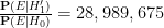
where is the likelihood of this information under the alternative hypothesis , and is the likelihood of this information under the null hypothesis . If there are no other hypotheses under consideration, then the two posterior probabilities , must add up to one, and so can be recovered from the posterior odds by the formulae

This gives a straightforward way to update one’s prior probabilities, and I thought I would present it in the form of a worksheet for ease of calculation:

A PDF version of the worksheet and instructions can be found here. One can fill in this worksheet in the following order:

1. In Box 1, one enters in the precise statement of the null hypothesis .
2. In Box 2, one enters in the precise statement of the alternative hypothesis . (This step is very important! As discussed in the previous post, Bayesian calculations can become extremely inaccurate if the alternative hypothesis is vague.)
3. In Box 3, one enters in the prior probability (or the best estimate thereof) of the null hypothesis .
4. In Box 4, one enters in the prior probability (or the best estimate thereof) of the alternative hypothesis . If only two hypotheses are being considered, we of course have .
5. In Box 5, one enters in the ratio between Box 4 and Box 3.
6. In Box 6, one enters in the precise new information that one has acquired since the prior state. (As discussed in the previous post, it is important that all relevant information – both supporting and invalidating the alternative hypothesis – are reported accurately. If one cannot be certain that key information has not been withheld to you, then Bayesian calculations become highly unreliable.)
7. In Box 7, one enters in the likelihood (or the best estimate thereof) of the new information under the null hypothesis .
8. In Box 8, one enters in the likelihood (or the best estimate thereof) of the new information under the null hypothesis . (This can be difficult to compute, particularly if is not specified precisely.)
9. In Box 9, one enters in the ratio betwen Box 8 and Box 7.
10. In Box 10, one enters in the product of Box 5 and Box 9.
11. (Assuming there are no other hypotheses than and ) In Box 11, enter in divided by plus Box 10.
12. (Assuming there are no other hypotheses than and ) In Box 12, enter in Box 10 divided by plus Box 10. (Alternatively, one can enter in minus Box 11.)

To illustrate this procedure, let us consider a standard Bayesian update problem. Suppose that a given point in time, of the population is infected with COVID-19. In response to this, a company mandates COVID-19 testing of its workforce, using a cheap COVID-19 test. This test has a chance of a false negative (testing negative when one has COVID) and a chance of a false positive (testing positive when one does not have COVID). An employee takes the mandatory test, which turns out to be positive. What is the probability that actually has COVID?

We can fill out the entries in the worksheet one at a time:

• Box 1: The null hypothesis is that does not have COVID.
• Box 2: The alternative hypothesis is that does have COVID.
• Box 3: In the absence of any better information, the prior probability of the null hypothesis is , or .
• Box 4: Similarly, the prior probability of the alternative hypothesis is , or .
• Box 5: The prior odds are .
• Box 6: The new information is that has tested positive for COVID.
• Box 7: The likelihood of under the null hypothesis is , or (the false positive rate).
• Box 8: The likelihood of under the alternative is , or (one minus the false negative rate).
• Box 9: The likelihood ratio is .
• Box 10: The product of Box 5 and Box 9 is approximately .
• Box 11: The posterior probability is approximately .
• Box 12: The posterior probability is approximately .

The filled worksheet looks like this:

Perhaps surprisingly, despite the positive COVID test, the employee only has a chance of actually having COVID! This is due to the relatively large false positive rate of this cheap test, and is an illustration of the base rate fallacy in statistics.

We remark that if we switch the roles of the null hypothesis and alternative hypothesis, then some of the odds in the worksheet change, but the ultimate conclusions remain unchanged:

So the question of which hypothesis to designate as the null hypothesis and which one to designate as the alternative hypothesis is largely a matter of convention.

Now let us take a superficially similar situation in which a mother observers her daughter exhibiting COVID-like symptoms, to the point where she estimates the probability of her daughter having COVID at . She then administers the same cheap COVID-19 test as before, which returns positive. What is the posterior probability of her daughter having COVID?

One can fill out the worksheet much as before, but now with the prior probability of the alternative hypothesis raised from to (and the prior probablity of the null hypothesis dropping from to ). One now gets that the probability that the daughter has COVID has increased all the way to :

Thus we see that prior probabilities can make a significant impact on the posterior probabilities.

Now we use the worksheet to analyze an infamous probability puzzle, the Monty Hall problem. Let us use the formulation given in that Wikipedia page:

Problem 1 Suppose you’re on a game show, and you’re given the choice of three doors: Behind one door is a car; behind the others, goats. You pick a door, say No. 1, and the host, who knows what’s behind the doors, opens another door, say No. 3, which has a goat. He then says to you, “Do you want to pick door No. 2?” Is it to your advantage to switch your choice?

For this problem, the precise formulation of the null hypothesis and the alternative hypothesis become rather important. Suppose we take the following two hypotheses:

• Null hypothesis : The car is behind door number 1, and no matter what door you pick, the host will randomly reveal another door that contains a goat.
• Alternative hypothesis : The car is behind door number 2 or 3, and no matter what door you pick, the host will randomly reveal another door that contains a goat.

Assuming the prizes are distributed randomly, we have and . The new information is that, after door 1 is selected, door 3 is revealed and shown to be a goat. After some thought, we conclude that is equal to (the host has a fifty-fifty chance of revealing door 3 instead of door 2) but that is also equal to (if the car is behind door 2, the host must reveal door 3, whereas if the car is behind door 3, the host cannot reveal door 3). Filling in the worksheet, we see that the new information does not in fact alter the odds, and the probability that the car is not behind door 1 remains at 2/3, so it is advantageous to switch.

However, consider the following different set of hypotheses:

• Null hypothesis : The car is behind door number 1, and if you pick the door with the car, the host will reveal another door to entice you to switch. Otherwise, the host will not reveal a door.
• Alternative hypothesis : The car is behind door number 2 or 3, and if you pick the door with the car, the host will reveal another door to entice you to switch. Otherwise, the host will not reveal a door.

Here we still have and , but while remains equal to , has dropped to zero (since if the car is not behind door 1, the host will not reveal a door). So now has increased all the way to , and it is not advantageous to switch! This dramatically illustrates the importance of specifying the hypotheses precisely. The worksheet is now filled out as follows:

Finally, we consider another famous probability puzzle, the Sleeping Beauty problem. Again we quote the problem as formulated on the Wikipedia page:

Problem 2 Sleeping Beauty volunteers to undergo the following experiment and is told all of the following details: On Sunday she will be put to sleep. Once or twice, during the experiment, Sleeping Beauty will be awakened, interviewed, and put back to sleep with an amnesia-inducing drug that makes her forget that awakening. A fair coin will be tossed to determine which experimental procedure to undertake:

• If the coin comes up heads, Sleeping Beauty will be awakened and interviewed on Monday only.
• If the coin comes up tails, she will be awakened and interviewed on Monday and Tuesday.
• In either case, she will be awakened on Wednesday without interview and the experiment ends.

Any time Sleeping Beauty is awakened and interviewed she will not be able to tell which day it is or whether she has been awakened before. During the interview Sleeping Beauty is asked: “What is your credence now for the proposition that the coin landed heads?”‘

Here the situation can be confusing because there are key portions of this experiment in which the observer is unconscious, but nevertheless Bayesian probability continues to operate regardless of whether the observer is conscious. To make this issue more precise, let us assume that the awakenings mentioned in the problem always occur at 8am, so in particular at 7am, Sleeping beauty will always be unconscious.

Here, the null and alternative hypotheses are easy to state precisely:

• Null hypothesis : The coin landed tails.
• Alternative hypothesis : The coin landed heads.

The subtle thing here is to work out what the correct prior state is (in most other applications of Bayesian probability, this state is obvious from the problem). It turns out that the most reasonable choice of prior state is “unconscious at 7am, on either Monday or Tuesday, with an equal chance of each”. (Note that whatever the outcome of the coin flip is, Sleeping Beauty will be unconscious at 7am Monday and unconscious again at 7am Tuesday, so it makes sense to give each of these two states an equal probability.) The new information is then

• New information : One hour after the prior state, Sleeping Beauty is awakened.

With this formulation, we see that , , and , so on working through the worksheet one eventually arrives at , so that Sleeping Beauty should only assign a probability of to the event that the coin landed as heads.

There are arguments advanced in the literature to adopt the position that should instead be equal to , but I do not see a way to interpret them in this Bayesian framework without a substantial alteration to either the notion of the prior state, or by not presenting the new information properly.

If one has multiple pieces of information that one wishes to use to update one’s priors, one can do so by filling out one copy of the worksheet for each new piece of information, or by using a multi-row version of the worksheet using such identities as

We leave the details of these variants of the Bayesian update problem to the interested reader. The only thing I will note though is that if a key piece of information is withheld from the person filling out the worksheet, for instance if that person relies exclusively on a news source that only reports information that supports the alternative hypothesis and omits information that debunks it, then the outcome of the worksheet is likely to be highly inaccurate, and one should only perform a Bayesian analysis when one has a high confidence that all relevant information (both favorable and unfavorable to the alternative hypothesis) is being reported to the user.

What are the odds?

An unusual lottery result made the news recently: on October 1, 2022, the PCSO Grand Lotto in the Philippines, which draws six numbers from to at random, managed to draw the numbers (though the balls were actually drawn in the order ). In other words, they drew exactly six multiples of nine from to . In addition, a total of tickets were bought with this winning combination, whose owners then had to split the million peso jackpot (about million USD) among themselves. This raised enough suspicion that there were calls for an inquiry into the Philippine lottery system, including from the minority leader of the Senate.

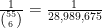
Whenever an event like this happens, journalists often contact mathematicians to ask the question: “What are the odds of this happening?”, and in fact I myself received one such inquiry this time around. This is a number that is not too difficult to compute – in this case, the probability of the lottery producing the six numbers in some order turn out to be in – and such a number is often dutifully provided to such journalists, who in turn report it as some sort of quantitative demonstration of how remarkable the event was.

But on the previous draw of the same lottery, on September 28, 2022, the unremarkable sequence of numbers were drawn (again in a different order), and no tickets ended up claiming the jackpot. The probability of the lottery producing the six numbers is also in – just as likely or as unlikely as the October 1 numbers . Indeed, the whole point of drawing the numbers randomly is to make each of the possible outcomes (whether they be “unusual” or “unremarkable”) equally likely. So why is it that the October 1 lottery attracted so much attention, but the September 28 lottery did not?

Part of the explanation surely lies in the unusually large number () of lottery winners on October 1, but I will set that aspect of the story aside until the end of this post. The more general points that I want to make with these sorts of situations are:

1. The question “what are the odds of happening” is often easy to answer mathematically, but it is not the correct question to ask.
2. The question “what is the probability that an alternative hypothesis is the truth” is (one of) the correct questions to ask, but is very difficult to answer (it involves both mathematical and non-mathematical considerations).
3. The answer to the first question is one of the quantities needed to calculate the answer to the second, but it is far from the only such quantity. Most of the other quantities involved cannot be calculated exactly.
4. However, by making some educated guesses, one can still sometimes get a very rough gauge of which events are “more surprising” than others, in that they would lead to relatively higher answers to the second question.

To explain these points it is convenient to adopt the framework of Bayesian probability. In this framework, one imagines that there are competing hypotheses to explain the world, and that one assigns a probability to each such hypothesis representing one’s belief in the truth of that hypothesis. For simplicity, let us assume that there are just two competing hypotheses to be entertained: the null hypothesis , and an alternative hypothesis . For instance, in our lottery example, the two hypotheses might be:

• Null hypothesis : The lottery is run in a completely fair and random fashion.
• Alternative hypothesis : The lottery is rigged by some corrupt officials for their personal gain.

At any given point in time, a person would have a probability assigned to the null hypothesis, and a probability assigned to the alternative hypothesis; in this simplified model where there are only two hypotheses under consideration, these probabilities must add to one, but of course if there were additional hypotheses beyond these two then this would no longer be the case.

Bayesian probability does not provide a rule for calculating the initial (or prior) probabilities , that one starts with; these may depend on the subjective experiences and biases of the person considering the hypothesis. For instance, one person might have quite a bit of prior faith in the lottery system, and assign the probabilities and . Another person might have quite a bit of prior cynicism, and perhaps assign and . One cannot use purely mathematical arguments to determine which of these two people is “correct” (or whether they are both “wrong”); it depends on subjective factors.

What Bayesian probability does do, however, is provide a rule to update these probabilities , in view of new information to provide posterior probabilities , . In our example, the new information would be the fact that the October 1 lottery numbers were (in some order). The update is given by the famous Bayes theorem

where is the probability that the event would have occurred under the null hypothesis , and is the probability that the event would have occurred under the alternative hypothesis . Let us divide the second equation by the first to cancel the denominator, and obtain

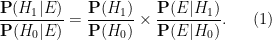
One can interpret as the prior odds of the alternative hypothesis, and as the posterior odds of the alternative hypothesis. The identity (1) then says that in order to compute the posterior odds of the alternative hypothesis in light of the new information , one needs to know three things:

1. The prior odds of the alternative hypothesis;
2. The probability that the event occurs under the null hypothesis ; and
3. The probability that the event occurs under the alternative hypothesis .

As previously discussed, the prior odds of the alternative hypothesis are subjective and vary from person to person; in the example earlier, the person with substantial faith in the lottery may only give prior odds of (99 to 1 against) of the alternative hypothesis, whereas the cynic might give odds of (even odds). The probability is the quantity that can often be calculated by straightforward mathematics; as discussed before, in this specific example we have

But this still leaves one crucial quantity that is unknown: the probability . This is incredibly difficult to compute, because it requires a precise theory for how events would play out under the alternative hypothesis , and in particular is very sensitive as to what the alternative hypothesis actually is.

For instance, suppose we replace the alternative hypothesis by the following very specific (and somewhat bizarre) hypothesis:

• Alternative hypothesis : The lottery is rigged by a cult that worships the multiples of , and views October 1 as their holiest day. On this day, they will manipulate the lottery to only select those balls that are multiples of .

Under this alternative hypothesis , we have . So, when happens, the odds of this alternative hypothesis will increase by the dramatic factor of . So, for instance, someone who already was entertaining odds of of this hypothesis would now have these odds multiply dramatically to , so that the probability of would have jumped from a mere to a staggering . This is about as strong a shift in belief as one could imagine. However, this hypothesis is so specific and bizarre that one’s prior odds of this hypothesis would be nowhere near as large as (unless substantial prior evidence of this cult and its hold on the lottery system existed, of course). A more realistic prior odds for would be something like – which is so miniscule that even multiplying it by a factor such as barely moves the needle.

Remark 1 The contrast between alternative hypothesis and alternative hypothesis illustrates a common demagogical rhetorical technique when an advocate is trying to convince an audience of an alternative hypothesis, namely to use suggestive language (“`I’m just asking questions here”) rather than precise statements in order to leave the alternative hypothesis deliberately vague. In particular, the advocate may take advantage of the freedom to use a broad formulation of the hypothesis (such as ) in order to maximize the audience’s prior odds of the hypothesis, simultaneously with a very specific formulation of the hypothesis (such as ) in order to maximize the probability of the actual event occuring under this hypothesis. (A related technique is to be deliberately vague about the hypothesized competency of some suspicious actor, so that this actor could be portrayed as being extraordinarily competent when convenient to do so, while simultaneously being portrayed as extraordinarily incompetent when that instead is the more useful hypothesis.) This can lead to wildly inaccurate Bayesian updates of this vague alternative hypothesis, and so precise formulation of such hypothesis is important if one is to approach a topic from anything remotely resembling a scientific approach. [EDIT: as pointed out to me by a reader, this technique is a Bayesian analogue of the motte and bailey fallacy.]

At the opposite extreme, consider instead the following hypothesis:

• Alternative hypothesis : The lottery is rigged by some corrupt officials, who on October 1 decide to randomly determine the winning numbers in advance, share these numbers with their collaborators, and then manipulate the lottery to choose those numbers that they selected.

If these corrupt officials are indeed choosing their predetermined winning numbers randomly, then the probability would in fact be just the same probability as , and in this case the seemingly unusual event would in fact have no effect on the odds of the alternative hypothesis, because it was just as unlikely for the alternative hypothesis to generate this multiples-of-nine pattern as for the null hypothesis to. In fact, one would imagine that these corrupt officials would avoid “suspicious” numbers, such as the multiples of , and only choose numbers that look random, in which case would in fact be less than and so the event would actually lower the odds of the alternative hypothesis in this case. (In fact, one can sometimes use this tendency of fraudsters to not generate truly random data as a statistical tool to detect such fraud; violations of Benford’s law for instance can be used in this fashion, though only in situations where the null hypothesis is expected to obey Benford’s law, as discussed in this previous blog post.)

Now let us consider a third alternative hypothesis:

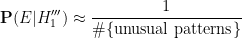
• Alternative hypothesis : On October 1, the lottery machine developed a fault and now only selects numbers that exhibit unusual patterns.

Setting aside the question of precisely what faulty mechanism could induce this sort of effect, it is not clear at all how to compute in this case. Using the principle of indifference as a crude rule of thumb, one might expect

where the denominator is the number of patterns among the possible lottery outcomes that are “unusual”. Among such patterns would presumably be the multiples-of-9 pattern 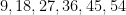, but one could easily come up with other patterns that are equally “unusual”, such as consecutive strings such as , or the first few primes , or the first few squares , and so forth. How many such unusual patterns are there? This is too vague a question to answer with any degree of precision, but as one illustrative statistic, the Online Encyclopedia of Integer Sequences (OEIS) currently hosts about sequences. Not all of these would begin with six distinct numbers from to , and several of these sequences might generate the same set of six numbers, but this does suggests that patterns that one would deem to be “unusual” could number in the thousands, tens of thousands, or more. Using this guess, we would then expect the event to boost the odds of this hypothesis by perhaps a thousandfold or so, which is moderately impressive. But subsequent information can counteract this effect. For instance, on October 3, the same lottery produced the numbers , which exhibit no unusual properties (no search results in the OEIS, for instance); if we denote this event by , then we have and so this new information should drive the odds for this alternative hypothesis way down again.

Remark 2 This example demonstrates another demagogical rhetorical technique that one sometimes sees (particularly in political or other emotionally charged contexts), which is to cherry-pick the information presented to their audience by informing them of events which have a relatively high probability of occurring under their alternative hypothesis, but withholding information about other relevant events that have a relatively low probability of occurring under their alternative hypothesis. When confronted with such new information , a common defense of a demogogue is to modify the alternative hypothesis to a more specific hypothesis that can “explain” this information (“Oh, clearly we heard about because the conspiracy in fact extends to the additional organizations that reported “), taking advantage of the vagueness discussed in Remark 1.

Let us consider a superficially similar hypothesis:

• Alternative hypothesis : On October 1, a divine being decided to send a sign to humanity by placing an unusual pattern in a lottery.

Here we (literally) stay agnostic on the prior odds of this hypothesis, and do not address the theological question of why a divine being should choose to use the medium of a lottery to send their signs. At first glance, the probability here should be similar to the probability , and so perhaps one could use this event to improve the odds of the existence of a divine being by a factor of a thousand or so. But note carefully that the hypothesis did not specify which lottery the divine being chose to use. The PSCO Grand Lotto is just one of a dozen lotteries run by the Philippine Charity Sweepstakes Office (PCSO), and of course there are over a hundred other countries and thousands of states within these countries, each of which often run their own lotteries. Taking into account these thousands or tens of thousands of additional lotteries to choose from, the probability now drops by several orders of magnitude, and is now basically comparable to the probability coming from the null hypothesis. As such one does not expect the event to have a significant impact on the odds of the hypothesis , despite the small-looking nature of the probability .

In summary, we have failed to locate any alternative hypothesis which

1. Has some non-negligible prior odds of being true (and in particular is not excessively specific, as with hypothesis );
2. Has a significantly higher probability of producing the specific event than the null hypothesis; AND
3. Does not struggle to also produce other events that have since been observed.

One needs all three of these factors to be present in order to significantly weaken the plausibility of the null hypothesis ; in the absence of these three factors, a moderately small numerical value of , such as does not actually do much to affect this plausibility. In this case one needs to lay out a reasonably precise alternative hypothesis and make some actual educated guesses towards the competing probability before one can lead to further conclusions. However, if is insanely small, e.g., less than , then the possibility of a previously overlooked alternative hypothesis becomes far more plausible; as per the famous quote of Arthur Conan Doyle’s Sherlock Holmes, “When you have eliminated all which is impossible, then whatever remains, however improbable, must be the truth.”

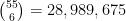
We now return to the fact that for this specific October 1 lottery, there were tickets that managed to select the winning numbers. Let us call this event . In view of this additional information, we should now consider the ratio of the probabilities and , rather than the ratio of the probabilities and . If we augment the null hypothesis to

• Null hypothesis : The lottery is run in a completely fair and random fashion, and the purchasers of lottery tickets also select their numbers in a completely random fashion.

Then is indeed of the “insanely improbable” category mentioned previously. I was not able to get official numbers on how many tickets are purchased per lottery, but let us say for sake of argument that it is 1 million (the conclusion will not be extremely sensitive to this choice). Then the expected number of tickets that would have the winning numbers would be

(which is broadly consistent, by the way, with the jackpot being reached every draws or so), and standard probability theory suggests that the number of winners should now follow a Poisson distribution with this mean . The probability of obtaining winners would now be

and of course would be even smaller than this. So this clearly demands some sort of explanation. But in actuality, many purchasers of lottery tickets do not select their numbers completely randomly; they often have some “lucky” numbers (e.g., based on birthdays or other personally significant dates) that they prefer to use, or choose numbers according to a simple pattern rather than go to the trouble of trying to make them truly random. So if we modify the null hypothesis to

• Null hypothesis : The lottery is run in a completely fair and random fashion, but a significant fraction of the purchasers of lottery tickets only select “unusual” numbers.

then it can now become quite plausible that a highly unusual set of numbers such as could be selected by as many as purchasers of tickets; for instance, if of the 1 million ticket holders chose to select their numbers according to some sort of pattern, then only of those holders would have to pick in order for the event to hold (given ), and this is not extremely implausible. Given that this reasonable version of the null hypothesis already gives a plausible explanation for , there does not seem to be a pressing need to locate an alternate hypothesis that gives some other explanation (cf. Occam’s razor). [UPDATE: Indeed, given the actual layout of the tickets of ths lottery, the numbers form a diagonal, and so all that is needed in order for the modified null hypothesis to explain the event is to postulate that a significant fraction of ticket purchasers decided to lay out their numbers in a simple geometric pattern, such as a row or diagonal.]

Remark 3 In view of the above discussion, one can propose a systematic way to evaluate (in as objective a fashion as possible) rhetorical claims in which an advocate is presenting evidence to support some alternative hypothesis:

1. State the null hypothesis and the alternative hypothesis as precisely as possible. In particular, avoid conflating an extremely broad hypothesis (such as the hypothesis in our running example) with an extremely specific one (such as in our example).
2. With the hypotheses precisely stated, give an honest estimate to the prior odds of this formulation of the alternative hypothesis.
3. Consider if all the relevant information (or at least a representative sample thereof) has been presented to you before proceeding further. If not, consider gathering more information from further sources.
4. Estimate how likely the information was to have occurred under the null hypothesis.
5. Estimate how likely the information was to have occurred under the alternative hypothesis (using exactly the same wording of this hypothesis as you did in previous steps).
6. If the second estimate is significantly larger than the first, then you have cause to update your prior odds of this hypothesis (though if those prior odds were already vanishingly unlikely, this may not move the needle significantly). If not, the argument is unconvincing and no significant adjustment to the odds (except perhaps in a downwards direction) needs to be made.