A small remark on the Elliott conjecture

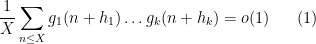
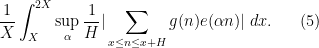
The Chowla conjecture asserts, among other things, that one has the asymptotic

as for any distinct integers , where is the Liouville function. (The usual formulation of the conjecture also allows one to consider more general linear forms than the shifts , but for sake of discussion let us focus on the shift case.) This conjecture remains open for , though there are now some partial results when one averages either in or in the , as discussed in this recent post.

A natural generalisation of the Chowla conjecture is the Elliott conjecture. Its original formulation was basically as follows: one had

whenever were bounded completely multiplicative functions and were distinct integers, and one of the was “non-pretentious” in the sense that

for all Dirichlet characters and real numbers . It is easy to see that some condition like (2) is necessary; for instance if and has period then can be verified to be bounded away from zero as .

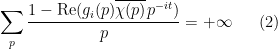
In a previous paper with Matomaki and Radziwill, we provided a counterexample to the original formulation of the Elliott conjecture, and proposed that (2) be replaced with the stronger condition

as for any Dirichlet character . To support this conjecture, we proved an averaged and non-asymptotic version of this conjecture which roughly speaking showed a bound of the form

whenever was an arbitrarily slowly growing function of , was sufficiently large (depending on and the rate at which grows), and one of the obeyed the condition

for some that was sufficiently large depending on , and all Dirichlet characters of period at most . As further support of this conjecture, I recently established the bound

under the same hypotheses, where is an arbitrarily slowly growing function of .

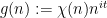
In view of these results, it is tempting to conjecture that the condition (4) for one of the should be sufficient to obtain the bound

when is large enough depending on . This may well be the case for . However, the purpose of this blog post is to record a simple counterexample for . Let’s take for simplicity. Let be a quantity much larger than but much smaller than (e.g. ), and set

For , Taylor expansion gives

and

and hence

and hence

On the other hand one can easily verify that all of the obey (4) (the restriction there prevents from getting anywhere close to ). So it seems the correct non-asymptotic version of the Elliott conjecture is the following:

Conjecture 1 (Non-asymptotic Elliott conjecture) Let be a natural number, and let be integers. Let , let be sufficiently large depending on , and let be sufficiently large depending on . Let be bounded multiplicative functions such that for some , one has

for all Dirichlet characters of conductor at most . Then

The case of this conjecture follows from the work of Halasz; in my recent paper a logarithmically averaged version of the case of this conjecture is established. The requirement to take to be as large as does not emerge in the averaged Elliott conjecture in my previous paper with Matomaki and Radziwill; it thus seems that this averaging has concealed some of the subtler features of the Elliott conjecture. (However, this subtlety does not seem to affect the asymptotic version of the conjecture formulated in that paper, in which the hypothesis is of the form (3), and the conclusion is of the form (1).)

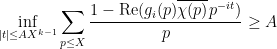
A similar subtlety arises when trying to control the maximal integral

In my previous paper with Matomaki and Radziwill, we could show that easier expression

was small (for a slowly growing function of ) if was bounded and completely multiplicative, and one had a condition of the form

for some large . However, to obtain an analogous bound for (5) it now appears that one needs to strengthen the above condition to

in order to address the counterexample in which for some between and . This seems to suggest that proving (5) (which is closely related to the case of the Chowla conjecture) could in fact be rather difficult; the estimation of (6) relied primarily of prior work of Matomaki and Radziwill which used the hypothesis (7), but as this hypothesis is not sufficient to conclude (5), some additional input must also be used.

275A, Notes 3: The weak and strong law of large numbers

One of the major activities in probability theory is studying the various statistics that can be produced from a complex system with many components. One of the simplest possible systems one can consider is a finite sequence or an infinite sequence of jointly independent scalar random variables, with the case when the are also identically distributed (i.e. the are iid) being a model case of particular interest. (In some cases one may consider a triangular array of scalar random variables, rather than a finite or infinite sequence.) There are many statistics of such sequences that one can study, but one of the most basic such statistics are the partial sums

The first fundamental result about these sums is the law of large numbers (or LLN for short), which comes in two formulations, weak (WLLN) and strong (SLLN). To state these laws, we first must define the notion of convergence in probability.

Definition 1 Let be a sequence of random variables taking values in a separable metric space (e.g. the could be scalar random variables, taking values in or ), and let be another random variable taking values in . We say that converges in probability to if, for every radius , one has as . Thus, if are scalar, we have converging to in probability if as for any given .

The measure-theoretic analogue of convergence in probability is convergence in measure.
It is instructive to compare the notion of convergence in probability with almost sure convergence. it is easy to see that converges almost surely to if and only if, for every radius , one has as ; thus, roughly speaking, convergence in probability is good for controlling how a single random variable is close to its putative limiting value , while almost sure convergence is good for controlling how the entire tail of a sequence of random variables is close to its putative limit .
We have the following easy relationships between convergence in probability and almost sure convergence:

Exercise 2 Let be a sequence of scalar random variables, and let be another scalar random variable.

• (i) If almost surely, show that in probability. Give a counterexample to show that the converse does not necessarily hold.
• (ii) Suppose that for all . Show that almost surely. Give a counterexample to show that the converse does not necessarily hold.
• (iii) If in probability, show that there is a subsequence of the such that almost surely.
• (iv) If are absolutely integrable and as , show that in probability. Give a counterexample to show that the converse does not necessarily hold.
• (v) (Urysohn subsequence principle) Suppose that every subsequence of has a further subsequence that converges to in probability. Show that also converges to in probability.
• (vi) Does the Urysohn subsequence principle still hold if “in probability” is replaced with “almost surely” throughout?
• (vii) If converges in probability to , and or is continuous, show that converges in probability to . More generally, if for each , is a sequence of scalar random variables that converge in probability to , and or is continuous, show that converges in probability to . (Thus, for instance, if and converge in probability to and respectively, then and converge in probability to and respectively.
• (viii) (Fatou’s lemma for convergence in probability) If are non-negative and converge in probability to , show that .
• (ix) (Dominated convergence in probability) If converge in probability to , and one almost surely has for all and some absolutely integrable , show that converges to .

Exercise 3 Let be a sequence of scalar random variables converging in probability to another random variable .

• (i) Suppose that there is a random variable which is independent of for each individual . Show that is also independent of .
• (ii) Suppose that the are jointly independent. Show that is almost surely constant (i.e. there is a deterministic scalar such that almost surely).

We can now state the weak and strong law of large numbers, in the model case of iid random variables.

Theorem 4 (Law of large numbers, model case) Let be an iid sequence of copies of an absolutely integrable random variable (thus the are independent and all have the same distribution as ). Write , and for each natural number , let denote the random variable .

• (i) (Weak law of large numbers) The random variables converge in probability to .
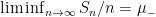
• (ii) (Strong law of large numbers) The random variables converge almost surely to .

Informally: if are iid with mean , then for large. Clearly the strong law of large numbers implies the weak law, but the weak law is easier to prove (and has somewhat better quantitative estimates). There are several variants of the law of large numbers, for instance when one drops the hypothesis of identical distribution, or when the random variable is not absolutely integrable, or if one seeks more quantitative bounds on the rate of convergence; we will discuss some of these variants below the fold.
It is instructive to compare the law of large numbers with what one can obtain from the Kolmogorov zero-one law, discussed in Notes 2. Observe that if the are real-valued, then the limit superior and are tail random variables in the sense that they are not affected if one changes finitely many of the ; in particular, events such as are tail events for any . From this and the zero-one law we see that there must exist deterministic quantities such that and almost surely. The strong law of large numbers can then be viewed as the assertion that when is absolutely integrable. On the other hand, the zero-one law argument does not require absolute integrability (and one can replace the denominator by other functions of that go to infinity as ).
The law of large numbers asserts, roughly speaking, that the theoretical expectation of a random variable can be approximated by taking a large number of independent samples of and then forming the empirical mean . This ability to approximate the theoretical statistics of a probability distribution through empirical data is one of the basic starting points for mathematical statistics, though this is not the focus of the course here. The tendency of statistics such as to cluster closely around their mean value is the simplest instance of the concentration of measure phenomenon, which is of tremendous significance not only within probability, but also in applications of probability to disciplines such as statistics, theoretical computer science, combinatorics, random matrix theory and high dimensional geometry. We will not discuss these topics much in this course, but see this previous blog post for some further discussion.
There are several ways to prove the law of large numbers (in both forms). One basic strategy is to use the moment method – controlling statistics such as by computing moments such as the mean , variance , or higher moments such as for . The joint independence of the make such moments fairly easy to compute, requiring only some elementary combinatorics. A direct application of the moment method typically requires one to make a finite moment assumption such as , but as we shall see, one can reduce fairly easily to this case by a truncation argument.
For the strong law of large numbers, one can also use methods relating to the theory of martingales, such as stopping time arguments and maximal inequalities; we present some classical arguments of Kolmogorov in this regard.

275A, Notes 2: Product measures and independence

In the previous set of notes, we constructed the measure-theoretic notion of the Lebesgue integral, and used this to set up the probabilistic notion of expectation on a rigorous footing. In this set of notes, we will similarly construct the measure-theoretic concept of a product measure (restricting to the case of probability measures to avoid unnecessary technicalities), and use this to set up the probabilistic notion of independence on a rigorous footing. (To quote Durrett: “measure theory ends and probability theory begins with the definition of independence.”) We will be able to take virtually any collection of random variables (or probability distributions) and couple them together to be independent via the product measure construction, though for infinite products there is the slight technicality (a requirement of the Kolmogorov extension theorem) that the random variables need to range in standard Borel spaces. This is not the only way to couple together such random variables, but it is the simplest and the easiest to compute with in practice, as we shall see in the next few sets of notes.

Sweeping a matrix rotates its graph

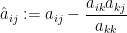
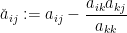
I recently learned about a curious operation on square matrices known as sweeping, which is used in numerical linear algebra (particularly in applications to statistics), as a useful and more robust variant of the usual Gaussian elimination operations seen in undergraduate linear algebra courses. Given an matrix (with, say, complex entries) and an index , with the entry non-zero, the sweep of at is the matrix given by the formulae

for all . Thus for instance if , and is written in block form as

for some row vector , column vector , and minor , one has

The inverse sweep operation is given by a nearly identical set of formulae:

for all . One can check that these operations invert each other. Actually, each sweep turns out to have order , so that : an inverse sweep performs the same operation as three forward sweeps. Sweeps also preserve the space of symmetric matrices (allowing one to cut down computational run time in that case by a factor of two), and behave well with respect to principal minors; a sweep of a principal minor is a principal minor of a sweep, after adjusting indices appropriately.

Remarkably, the sweep operators all commute with each other: . If and we perform the first sweeps (in any order) to a matrix

with a minor, a matrix, a matrix, and a matrix, one obtains the new matrix

Note the appearance of the Schur complement in the bottom right block. Thus, for instance, one can essentially invert a matrix by performing all sweeps:

If a matrix has the form

for a minor , column vector , row vector , and scalar , then performing the first sweeps gives

and all the components of this matrix are usable for various numerical linear algebra applications in statistics (e.g. in least squares regression). Given that sweeps behave well with inverses, it is perhaps not surprising that sweeps also behave well under determinants: the determinant of can be factored as the product of the entry and the determinant of the matrix formed from by removing the row and column. As a consequence, one can compute the determinant of fairly efficiently (so long as the sweep operations don’t come close to dividing by zero) by sweeping the matrix for in turn, and multiplying together the entry of the matrix just before the sweep for to obtain the determinant.

It turns out that there is a simple geometric explanation for these seemingly magical properties of the sweep operation. Any matrix creates a graph (where we think of as the space of column vectors). This graph is an -dimensional subspace of . Conversely, most subspaces of arises as graphs; there are some that fail the vertical line test, but these are a positive codimension set of counterexamples.

We use to denote the standard basis of , with the standard basis for the first factor of and the standard basis for the second factor. The operation of sweeping the entry then corresponds to a ninety degree rotation in the plane, that sends to (and to ), keeping all other basis vectors fixed: thus we have

for generic (more precisely, those with non-vanishing entry ). For instance, if and is of the form (1), then is the set of tuples obeying the equations

The image of under is . Since we can write the above system of equations (for ) as

we see from (2) that is the graph of . Thus the sweep operation is a multidimensional generalisation of the high school geometry fact that the line in the plane becomes after applying a ninety degree rotation.

It is then an instructive exercise to use this geometric interpretation of the sweep operator to recover all the remarkable properties about these operations listed above. It is also useful to compare the geometric interpretation of sweeping as rotation of the graph to that of Gaussian elimination, which instead shears and reflects the graph by various elementary transformations (this is what is going on geometrically when one performs Gaussian elimination on an augmented matrix). Rotations are less distorting than shears, so one can see geometrically why sweeping can produce fewer numerical artefacts than Gaussian elimination.

275A, Notes 1: Integration and expectation

In Notes 0, we introduced the notion of a measure space , which includes as a special case the notion of a probability space. By selecting one such probability space as a sample space, one obtains a model for random events and random variables, with random events being modeled by measurable sets in , and random variables taking values in a measurable space being modeled by measurable functions . We then defined some basic operations on these random events and variables:

• Given events , we defined the conjunction , the disjunction , and the complement . For countable families of events, we similarly defined and . We also defined the empty event and the sure event , and what it meant for two events to be equal.
• Given random variables in ranges respectively, and a measurable function , we defined the random variable in range . (As the special case of this, every deterministic element of was also a random variable taking values in .) Given a relation , we similarly defined the event . Conversely, given an event , we defined the indicator random variable . Finally, we defined what it meant for two random variables to be equal.
• Given an event , we defined its probability .

These operations obey various axioms; for instance, the boolean operations on events obey the axioms of a Boolean algebra, and the probabilility function obeys the Kolmogorov axioms. However, we will not focus on the axiomatic approach to probability theory here, instead basing the foundations of probability theory on the sample space models as discussed in Notes 0. (But see this previous post for a treatment of one such axiomatic approach.)

It turns out that almost all of the other operations on random events and variables we need can be constructed in terms of the above basic operations. In particular, this allows one to safely extend the sample space in probability theory whenever needed, provided one uses an extension that respects the above basic operations; this is an important operation when one needs to add new sources of randomness to an existing system of events and random variables, or to couple together two separate such systems into a joint system that extends both of the original systems. We gave a simple example of such an extension in the previous notes, but now we give a more formal definition:

Definition 1 Suppose that we are using a probability space as the model for a collection of events and random variables. An extension of this probability space is a probability space , together with a measurable map (sometimes called the factor map) which is probability-preserving in the sense that

for all . (Caution: this does not imply that for all – why not?)

An event which is modeled by a measurable subset in the sample space , will be modeled by the measurable set in the extended sample space . Similarly, a random variable taking values in some range that is modeled by a measurable function in , will be modeled instead by the measurable function in . We also allow the extension to model additional events and random variables that were not modeled by the original sample space (indeed, this is one of the main reasons why we perform extensions in probability in the first place).

Thus, for instance, the sample space in Example 3 of the previous post is an extension of the sample space in that example, with the factor map given by the first coordinate projection . One can verify that all of the basic operations on events and random variables listed above are unaffected by the above extension (with one caveat, see remark below). For instance, the conjunction of two events can be defined via the original model by the formula

or via the extension via the formula

The two definitions are consistent with each other, thanks to the obvious set-theoretic identity

Similarly, the assumption (1) is precisely what is needed to ensure that the probability of an event remains unchanged when one replaces a sample space model with an extension. We leave the verification of preservation of the other basic operations described above under extension as exercises to the reader.

Remark 2 There is one minor exception to this general rule if we do not impose the additional requirement that the factor map is surjective. Namely, for non-surjective , it can become possible that two events are unequal in the original sample space model, but become equal in the extension (and similarly for random variables), although the converse never happens (events that are equal in the original sample space always remain equal in the extension). For instance, let be the discrete probability space with and , and let be the discrete probability space with , and non-surjective factor map defined by . Then the event modeled by in is distinct from the empty event when viewed in , but becomes equal to that event when viewed in . Thus we see that extending the sample space by a non-surjective factor map can identify previously distinct events together (though of course, being probability preserving, this can only happen if those two events were already almost surely equal anyway). This turns out to be fairly harmless though; while it is nice to know if two given events are equal, or if they differ by a non-null event, it is almost never useful to know that two events are unequal if they are already almost surely equal. Alternatively, one can add the additional requirement of surjectivity in the definition of an extension, which is also a fairly harmless constraint to impose (this is what I chose to do in this previous set of notes).

Roughly speaking, one can define probability theory as the study of those properties of random events and random variables that are model-independent in the sense that they are preserved by extensions. For instance, the cardinality of the model of an event is not a concept within the scope of probability theory, as it is not preserved by extensions: continuing Example 3 from Notes 0, the event that a die roll is even is modeled by a set of cardinality in the original sample space model , but by a set of cardinality in the extension. Thus it does not make sense in the context of probability theory to refer to the “cardinality of an event “.

On the other hand, the supremum of a collection of random variables in the extended real line is a valid probabilistic concept. This can be seen by manually verifying that this operation is preserved under extension of the sample space, but one can also see this by defining the supremum in terms of existing basic operations. Indeed, note from Exercise 24 of Notes 0 that a random variable in the extended real line is completely specified by the threshold events for ; in particular, two such random variables are equal if and only if the events and are surely equal for all . From the identity

we thus see that one can completely specify in terms of using only the basic operations provided in the above list (and in particular using the countable conjunction .) Of course, the same considerations hold if one replaces supremum, by infimum, limit superior, limit inferior, or (if it exists) the limit.

In this set of notes, we will define some further important operations on scalar random variables, in particular the expectation of these variables. In the sample space models, expectation corresponds to the notion of integration on a measure space. As we will need to use both expectation and integration in this course, we will thus begin by quickly reviewing the basics of integration on a measure space, although we will then translate the key results of this theory into probabilistic language.

As the finer details of the Lebesgue integral construction are not the core focus of this probability course, some of the details of this construction will be left to exercises. See also Chapter 1 of Durrett, or these previous blog notes, for a more detailed treatment.