
You are currently browsing the monthly archive for June 2013.
For any 
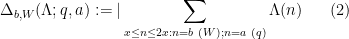
![{B[H]}](https://s0.wp.com/latex.php?latex=%7BB%5BH%5D%7D&bg=ffffff&fg=000000&s=0&c=20201002)


thus for instance ![{B[2]}](https://s0.wp.com/latex.php?latex=%7BB%5B2%5D%7D&bg=ffffff&fg=000000&s=0&c=20201002)
Theorem 1 (Zhang’s theorem)
In fact, Zhang’s paper shows that 
About a month ago, the Polymath8 project was launched with the objective of reading through Zhang’s paper, clarifying the arguments, and then making them more efficient, in order to improve the value of 

The precise arguments here are quite technical, and are discussed at length on other posts on this blog. In this post, I would like to give a “high level” summary of how Zhang’s argument works, and give some impressions of the improvements we have made so far; these would already be familiar to the active participants of the Polymath8 project, but perhaps may be of value to people who are following this project on a more casual basis.
While Zhang’s arguments (and our refinements of it) are quite lengthy, they are fortunately also very modular, that is to say they can be broken up into several independent components that can be understood and optimised more or less separately from each other (although we have on occasion needed to modify the formulation of one component in order to better suit the needs of another). At the top level, Zhang’s argument looks like this:
- Statements of the form
(the
stands for “Dickson-Hardy-Littlewood”), by locating suitable narrow admissible tuples (see below). Zhang’s paper establishes for the first time an unconditional proof of
; in his initial paper,
, but we have lowered this value to
(and provisionally to
). Any reduction in the value of
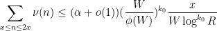
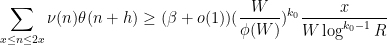
- Next, by adapting sieve-theoretic arguments of Goldston, Pintz, and Yildirim, the Dickson-Hardy-Littlewood type assertions
(the
stands for “Motohashi-Pintz-Zhang”). More recently, we have replaced the conjecture
to significantly improve the efficiency of this step (using some recent ideas of Pintz). Roughly speaking, these statements assert that the primes are more or less evenly distributed along many arithmetic progressions, including those that have relatively large spacing. A crucial technical fact here is that in contrast to the older Elliott-Halberstam conjecture, the Motohashi-Pintz-Zhang estimates only require one to control progressions whose spacings
have a lot of small prime factors (the original
parameter is more important than the technical parameter
; we would like
; we have now increased this to be almost as large as
(and provisionally
).
- By a certain amount of combinatorial manipulation (combined with a useful decomposition of the von Mangoldt function due Heath-Brown), estimates such as
, the “Type II” estimate
, and the “Type III” estimate
, which all involve the distribution of certain Dirichlet convolutions in arithmetic progressions. Here
is an adjustable parameter that demarcates the border between the Type I and Type III estimates; raising
makes it easier to prove Type III estimates but harder to prove Type I estimates, and lowering
and
for which all three estimates
arises from the combinatorics, and appears to be rather essential; in fact, it is currently a major obstacle to further improvement of
- The Type I estimates
, where
are moderately long sequences which have controlled magnitude and length but are otherwise arbitrary. Estimates that are roughly of this type first appeared in a series of papers by Bombieri, Fouvry, Friedlander, Iwaniec, and other authors, and Zhang’s arguments here broadly follow those of previous authors, but with several new twists that take advantage of the many factors of the spacing
Zhang’s argument uses classical estimates on this Kloosterman sum (dating back to the work of Weil), but we have improved this using the “
-process” introduced by Heath-Brown and Ringrose.
- The Type II estimates
than the other two estimates, and so as a first approximation one can ignore the need to treat these estimates, although recently our Type I and Type III estimates have become so strong that it has become necessary to tighten the Type II estimates as well.
- The Type III estimates
in arithmetic progressions. There are various ways to attack this problem, but most of them ultimately boil down (after the use of standard devices such as Cauchy-Schwarz and completion of sums) to the task of controlling certain higher-dimensional Kloosterman-type sums such as
In principle, any such sum can be controlled by invoking Deligne’s proof of the Weil conjectures in arbitrary dimension (which, roughly speaking, establishes the analogue of the Riemann hypothesis for arbitrary varieties over finite fields), although in the higher dimensional setting some algebraic geometry is needed to ensure that one gets the full “square root cancellation” for these exponential sums. (For the particular sum above, the necessary details were worked out by Birch and Bombieri.) As such, this part of the argument is by far the least elementary component of the whole. Zhang’s original argument cleverly exploited some additional cancellation in the above exponential sums that goes beyond the naive square root cancellation heuristic; more recently, an alternate argument of Fouvry, Kowalski, Michel, and Nelson uses bounds on a slightly different higher-dimensional Kloosterman-type sum to obtain results that give better values of
. We have also been able to improve upon these estimates by exploiting some additional averaging that was left unused by the previous arguments.


As of this time of writing, our understanding of the first three stages of Zhang’s argument (getting from
Below the fold I will discuss (mostly at an informal, non-rigorous level) the six steps above in a little more detail (full details can of course be found in the other polymath8 posts on this blog). This post will also serve as a new research thread, as the previous threads were getting quite lengthy.
As in previous posts, we use the following asymptotic notation: 


The purpose of this post is to collect together all the various refinements to the second half of Zhang’s paper that have been obtained as part of the polymath8 project and present them as a coherent argument (though not fully self-contained, as we will need some lemmas from previous posts).
In order to state the main result, we need to recall some definitions.
Definition 1 (Singleton congruence class system) Let
, and let
denote the square-free numbers whose prime factors lie in
. A singleton congruence class system on
of primitive residue classes
for each
, obeying the Chinese remainder theorem property
whenever
are coprime. We say that such a system
has controlled multiplicity if the
for any fixed
and any congruence class
with
. Here
is the divisor function.


Next we need a relaxation of the concept of 
Definition 2 (Dense divisibility) Let
. A positive integer
, there exists a factor of
. We let
denote the set of
Now we present a strengthened version 

Conjecture 3 (
be a congruence class system with controlled multiplicity. Then
for any fixed
, where
is the von Mangoldt function.
![\displaystyle \sum_{q \in {\mathcal S}_I \cap {\mathcal D}_{x^\delta}: q< x^{1/2+2\varpi}} |\Delta(\Lambda 1_{[x,2x]}; a_q)| \ll x \log^{-A} x \ \ \ \ \ (3)](https://s0.wp.com/latex.php?latex=%5Cdisplaystyle++%5Csum_%7Bq+%5Cin+%7B%5Cmathcal+S%7D_I+%5Ccap+%7B%5Cmathcal+D%7D_%7Bx%5E%5Cdelta%7D%3A+q%3C+x%5E%7B1%2F2%2B2%5Cvarpi%7D%7D+%7C%5CDelta%28%5CLambda+1_%7B%5Bx%2C2x%5D%7D%3B+a_q%29%7C+%5Cll+x+%5Clog%5E%7B-A%7D+x+%5C+%5C+%5C+%5C+%5C+%283%29&bg=ffffff&fg=000000&s=0&c=20201002)
The difference between this conjecture and the weaker conjecture 
![{[1,x^\delta]}](https://s0.wp.com/latex.php?latex=%7B%5B1%2Cx%5E%5Cdelta%5D%7D&bg=ffffff&fg=000000&s=0&c=20201002)
The main result we will establish is
 with
with 
This improves upon previous constraints of 


As in previous posts, we use the following asymptotic notation: 
This post is intended to highlight a phenomenon unearthed in the ongoing polymath8 project (and is in fact a key component of Zhang’s proof that there are bounded gaps between primes infinitely often), namely that one can get quite good bounds on relatively short exponential sums when the modulus
To illustrate the method, let us begin with the classical problem in analytic number theory of estimating an incomplete character sum
where 


we also have the classical Pólya-Vinogradov inequality

This latter inequality gives improvements over the trivial bound when 

for any 


In the case when

to the Pólya-Vinogradov inequality when 
Another important improvement is the Burgess bound, which in our notation asserts that
for any fixed integer 

In the case when 

However, in the opposite case when
Proposition 1 Let
and of polynomial size, and let
be integers with
. Then for any primitive character

This proposition is particularly powerful when 


which can improve upon the Burgess bound when 


The hypothesis that
Proof: If 


We use the method of Weyl differencing, the key point being to difference in multiples of
Let 


![\displaystyle \sum_{M+1 \leq n \leq M+N} \chi(n) = \sum_n 1_{[M+1,M+N]}(n+kq_1) \chi(n+kq_1)](https://s0.wp.com/latex.php?latex=%5Cdisplaystyle++%5Csum_%7BM%2B1+%5Cleq+n+%5Cleq+M%2BN%7D+%5Cchi%28n%29+%3D+%5Csum_n+1_%7B%5BM%2B1%2CM%2BN%5D%7D%28n%2Bkq_1%29+%5Cchi%28n%2Bkq_1%29&bg=ffffff&fg=000000&s=0&c=20201002)
![\displaystyle \sum_{M+1 \leq n \leq M+N} \chi(n) = \frac{1}{K} \sum_n \sum_{k=1}^K 1_{[M+1,M+N]}(n+kq_1) \chi(n+kq_1). \ \ \ \ \ (4)](https://s0.wp.com/latex.php?latex=%5Cdisplaystyle++%5Csum_%7BM%2B1+%5Cleq+n+%5Cleq+M%2BN%7D+%5Cchi%28n%29+%3D+%5Cfrac%7B1%7D%7BK%7D+%5Csum_n+%5Csum_%7Bk%3D1%7D%5EK+1_%7B%5BM%2B1%2CM%2BN%5D%7D%28n%2Bkq_1%29+%5Cchi%28n%2Bkq_1%29.+%5C+%5C+%5C+%5C+%5C+%284%29&bg=ffffff&fg=000000&s=0&c=20201002)
By the Chinese remainder theorem, we may factor
where 


and so we can take
![\displaystyle \sum_{M+1 \leq n \leq M+N} \chi(n) = \frac{1}{K} \sum_n \chi_1(n) \sum_{k=1}^K 1_{[M+1,M+N]}(n+kq_1) \chi_2(n+kq_1)](https://s0.wp.com/latex.php?latex=%5Cdisplaystyle++%5Csum_%7BM%2B1+%5Cleq+n+%5Cleq+M%2BN%7D+%5Cchi%28n%29+%3D+%5Cfrac%7B1%7D%7BK%7D+%5Csum_n+%5Cchi_1%28n%29+%5Csum_%7Bk%3D1%7D%5EK+1_%7B%5BM%2B1%2CM%2BN%5D%7D%28n%2Bkq_1%29+%5Cchi_2%28n%2Bkq_1%29+&bg=ffffff&fg=000000&s=0&c=20201002)
and hence by the triangle inequality
![\displaystyle |\sum_{M+1 \leq n \leq M+N} \chi(n)| \leq \frac{1}{K} \sum_n |\sum_{k=1}^K 1_{[M+1,M+N]}(n+kq_1) \chi_2(n+kq_1)|.](https://s0.wp.com/latex.php?latex=%5Cdisplaystyle++%7C%5Csum_%7BM%2B1+%5Cleq+n+%5Cleq+M%2BN%7D+%5Cchi%28n%29%7C+%5Cleq+%5Cfrac%7B1%7D%7BK%7D+%5Csum_n+%7C%5Csum_%7Bk%3D1%7D%5EK+1_%7B%5BM%2B1%2CM%2BN%5D%7D%28n%2Bkq_1%29+%5Cchi_2%28n%2Bkq_1%29%7C.+&bg=ffffff&fg=000000&s=0&c=20201002)
Note how the characters on the right-hand side only have period 

Note that the inner sum vanishes unless ![{n \in [M+1-Kq_1,M+N]}](https://s0.wp.com/latex.php?latex=%7Bn+%5Cin+%5BM%2B1-Kq_1%2CM%2BN%5D%7D&bg=ffffff&fg=000000&s=0&c=20201002)


![\displaystyle \frac{N^{1/2}}{K} (\sum_n |\sum_{k=1}^K 1_{[M+1,M+N]}(n+kq_1) \chi_2(n+kq_1)|^2)^{1/2}.](https://s0.wp.com/latex.php?latex=%5Cdisplaystyle++%5Cfrac%7BN%5E%7B1%2F2%7D%7D%7BK%7D+%28%5Csum_n+%7C%5Csum_%7Bk%3D1%7D%5EK+1_%7B%5BM%2B1%2CM%2BN%5D%7D%28n%2Bkq_1%29+%5Cchi_2%28n%2Bkq_1%29%7C%5E2%29%5E%7B1%2F2%7D.&bg=ffffff&fg=000000&s=0&c=20201002)
We expand the right-hand side as

![\displaystyle 1_{[M+1,M+N]}(n+kq_1) 1_{[M+1,M+N]}(n+k'q_1) \chi_2(n+kq_1) \overline{\chi_2(n+k'q_1)}|^{1/2}.](https://s0.wp.com/latex.php?latex=%5Cdisplaystyle++1_%7B%5BM%2B1%2CM%2BN%5D%7D%28n%2Bkq_1%29+1_%7B%5BM%2B1%2CM%2BN%5D%7D%28n%2Bk%27q_1%29+%5Cchi_2%28n%2Bkq_1%29+%5Coverline%7B%5Cchi_2%28n%2Bk%27q_1%29%7D%7C%5E%7B1%2F2%7D.&bg=ffffff&fg=000000&s=0&c=20201002)
We first consider the diagonal contribution 
Now we consider the off-diagonal case; by symmetry we can take 
![{1_{[M+1,M+N]}(n+kq_1) 1_{[M+1,M+N]}(n+k'q_1)}](https://s0.wp.com/latex.php?latex=%7B1_%7B%5BM%2B1%2CM%2BN%5D%7D%28n%2Bkq_1%29+1_%7B%5BM%2B1%2CM%2BN%5D%7D%28n%2Bk%27q_1%29%7D&bg=ffffff&fg=000000&s=0&c=20201002)

![{[M+1-kq_1, M+N-k'q_1]}](https://s0.wp.com/latex.php?latex=%7B%5BM%2B1-kq_1%2C+M%2BN-k%27q_1%5D%7D&bg=ffffff&fg=000000&s=0&c=20201002)

for any 
![\displaystyle |\sum_n 1_{[M+1,M+N]}(n+kq_1) 1_{[M+1,M+N]}(n+k'q_1) \chi_2(n+kq_1) \overline{\chi_2(n+k'q_1)}|](https://s0.wp.com/latex.php?latex=%5Cdisplaystyle++%7C%5Csum_n+1_%7B%5BM%2B1%2CM%2BN%5D%7D%28n%2Bkq_1%29+1_%7B%5BM%2B1%2CM%2BN%5D%7D%28n%2Bk%27q_1%29+%5Cchi_2%28n%2Bkq_1%29+%5Coverline%7B%5Cchi_2%28n%2Bk%27q_1%29%7D%7C+&bg=ffffff&fg=000000&s=0&c=20201002)
Summing in 

which simplifies to 

A modification of the above argument (using more complicated versions of the Weil conjectures) allows one to replace the summand 


where 
This post is a continuation of the previous post on sieve theory, which is an ongoing part of the Polymath8 project. As the previous post was getting somewhat full, we are rolling the thread over to the current post.
In this post we will record a new truncation of the elementary Selberg sieve discussed in this previous post (and also analysed in the context of bounded prime gaps by Graham-Goldston-Pintz-Yildirim and Motohashi-Pintz) that was recently worked out by Janos Pintz, who has kindly given permission to share this new idea with the Polymath8 project. This new sieve decouples the 

To describe this new truncation we need to review some notation. As in all previous posts (in particular, the first post in this series), we have an asymptotic parameter 


For any fixed natural number 

Conjecture 1 (
of
The twin prime conjecture asserts that 

In previous posts, we deduced 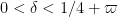
Conjecture 2 (
, and let
be a primitive residue class. Then
for any fixed
,
is the quantity
and
is the set of congruence classes
and
is the polynomial


The conjecture 
To connect the two conjectures, the previously best known implication was the folowing (see Theorem 2 from this post):
Theorem 3 Let
and
where
is the first positive zero of the Bessel function
, and
are the quantities
and
Then


Actually there have been some slight improvements to the quantities 

To improve beyond this, the first basic observation is that the smoothness condition
Definition 4 Let
. A positive integer
Certainly every integer which is
We now define 
The main result of this post is then the following implication, essentially due to Pintz:
Theorem 5 Let
,
, and
where
and
and
Then


This theorem has rather messy constants, but we can isolate some special cases which are a bit easier to compute with. Setting 

Theorem 6 Let
where
Then


This is a little better than Theorem 3, because the error 


Returning to the full strength of Theorem 5, let us obtain a crude upper bound for 

We can crudely bound

and then optimise in
Because of the 


Pintz’s argument uses the elementary Selberg sieve, discussed in this previous post, but with a more efficient estimation of the quantity 


This is the final continuation of the online reading seminar of Zhang’s paper for the polymath8 project. (There are two other continuations; this previous post, which deals with the combinatorial aspects of the second part of Zhang’s paper, and this previous post, that covers the Type I and Type II sums.) The main purpose of this post is to present (and hopefully, to improve upon) the treatment of the final and most innovative of the key estimates in Zhang’s paper, namely the Type III estimate.
The main estimate was already stated as Theorem 17 in the previous post, but we quickly recall the relevant definitions here. As in other posts, we always take
Definition 1 (Coefficient sequences) A coefficient sequence is a finitely supported sequence
that obeys the bounds
for all
- (i) If
is a coefficient sequence and
is a primitive residue class, the (signed) discrepancy
of
- (ii) A coefficient sequence
if it is supported on an interval of the form
.
- (iii) A coefficient sequence
for some smooth function
supported on
obeying the derivative bounds
for all fixed
(note that the implied constant in the
notation may depend on
).


For any
Theorem 2 (Type III estimate) Let
be fixed quantities, and let
be quantities such that
and
and
for some fixed
. Let
be coefficient sequences at scale
respectively with
smooth. Then for any
we have
In fact we have the stronger “pointwise” estimate
for all
and all
, and some fixed
.


(This is very slightly stronger than previously claimed, in that the condition 
It turns out that Zhang does not exploit any averaging of the
Theorem 3 (Type III estimate without
be fixed, and let
be quantities such that
and
and
for some fixed
respectively. Then we have
for all
and some fixed

![\displaystyle d \in {\mathcal S}_{[1,x^\delta]}](https://s0.wp.com/latex.php?latex=%5Cdisplaystyle+d+%5Cin+%7B%5Cmathcal+S%7D_%7B%5B1%2Cx%5E%5Cdelta%5D%7D&bg=ffffff&fg=000000&s=0&c=20201002)


Let us quickly see how Theorem 3 implies Theorem 2. To show (4), it suffices to establish the bound

for all 


From Theorem 3 we have

where the quantity 


It remains to establish Theorem 3. This is done by a set of tools similar to that used to control the Type I and Type II sums:
- (i) completion of sums;
- (ii) the Weil conjectures and bounds on Ramanujan sums;
- (iii) factorisation of smooth moduli
- (iv) the Cauchy-Schwarz and triangle inequalities (Weyl differencing).
The specifics are slightly different though. For the Type I and Type II sums, it was the classical Weil bound on Kloosterman sums that were the key source of power saving; Ramanujan sums only played a minor role, controlling a secondary error term. For the Type III sums, one needs a significantly deeper consequence of the Weil conjectures, namely the estimate of Bombieri and Birch on a three-dimensional variant of a Kloosterman sum. Furthermore, the Ramanujan sums – which are a rare example of sums that actually exhibit better than square root cancellation, thus going beyond even what the Weil conjectures can offer – make a crucial appearance, when combined with the factorisation of the smooth modulus
Tamar Ziegler and I have just uploaded to the arXiv our joint paper “A multi-dimensional Szemerédi theorem for the primes via a correspondence principle“. This paper is related to an earlier result of Ben Green and mine in which we established that the primes contain arbitrarily long arithmetic progressions. Actually, in that paper we proved a more general result:
Theorem 1 (Szemerédi’s theorem in the primes) Let
of positive relative density, thus
. Then
This result was based in part on an earlier paper of Green that handled the case of progressions of length three. With the primes replaced by the integers, this is of course the famous theorem of Szemerédi.
Szemerédi’s theorem has now been generalised in many different directions. One of these is the multidimensional Szemerédi theorem of Furstenberg and Katznelson, who used ergodic-theoretic techniques to show that any dense subset of 
Theorem 2 (Multidimensional Szemerédi theorem in the primes) Let
, and let
Cartesian power
of the primes of positive relative density, thus
Then for any
,
with
and
![\displaystyle \limsup_{N \rightarrow \infty} \frac{|A \cap [N]^d|}{|{\mathcal P}^d \cap [N]^d|} > 0.](https://s0.wp.com/latex.php?latex=%5Cdisplaystyle++%5Climsup_%7BN+%5Crightarrow+%5Cinfty%7D+%5Cfrac%7B%7CA+%5Ccap+%5BN%5D%5Ed%7C%7D%7B%7C%7B%5Cmathcal+P%7D%5Ed+%5Ccap+%5BN%5D%5Ed%7C%7D+%3E+0.&bg=ffffff&fg=000000&s=0&c=20201002)
In the case when
The result is reminiscent of an earlier result of mine on finding constellations in the Gaussian primes (or dense subsets thereof). That paper followed closely the arguments of my original paper with Ben Green, namely it first enclosed (a W-tricked version of) the primes or Gaussian primes (in a sieve theoretic-sense) by a slightly larger set (or more precisely, a weight function 

However, when one tries to adapt these arguments to sets such as 


do not behave independently (as they would if 
There are now two ways known to get around this problem and establish Theorem 2 in full generality. The approach of Cook, Magyar, and Titichetrakun proceeds by starting with one of the known proofs of the multidimensional Szemerédi theorem – namely, the proof that proceeds through hypergraph regularity and hypergraph removal – and attach pseudorandom weights directly within the proof itself, rather than trying to add the weights to the result of that proof through a transference argument. (A key technical issue is that weights have to be added to all the levels of the hypergraph – not just the vertices and top-order edges – in order to circumvent the failure of naive pseudorandomness.) As one has to modify the entire proof of the multidimensional Szemerédi theorem, rather than use that theorem as a black box, the Cook-Magyar-Titichetrakun argument is lengthier than ours; on the other hand, it is more general and does not rely on some difficult theorems about primes that are used in our paper.
In our approach, we continue to use the multidimensional Szemerédi theorem (or more precisely, the equivalent theorem of Furstenberg and Katznelson concerning multiple recurrence for commuting shifts) as a black box. The difference is that instead of using a transference principle to connect the relative multidimensional Szemerédi theorem we need to the multiple recurrence theorem, we instead proceed by a version of the Furstenberg correspondence principle, similar to the one that connects the absolute multidimensional Szemerédi theorem to the multiple recurrence theorem. I had discovered this approach many years ago in an unpublished note, but had abandoned it because it required an infinite number of linear forms conditions (in contrast to the transference technique, which only needed a finite number of linear forms conditions and (until the recent work of Conlon-Fox-Zhao) a correlation condition). The reason for this infinite number of conditions is that the correspondence principle has to build a probability measure on an entire 


With the sieve weights
This is one of the continuations of the online reading seminar of Zhang’s paper for the polymath8 project. (There are two other continuations; this previous post, which deals with the combinatorial aspects of the second part of Zhang’s paper, and a post to come that covers the Type III sums.) The main purpose of this post is to present (and hopefully, to improve upon) the treatment of two of the three key estimates in Zhang’s paper, namely the Type I and Type II estimates.
The main estimate was already stated as Theorem 16 in the previous post, but we quickly recall the relevant definitions here. As in other posts, we always take
Definition 1 (Coefficient sequences) A coefficient sequence is a finitely supported sequence
for all
- (i) If
- (ii) A coefficient sequence
- (iii) A coefficient sequence
for any
, any fixed
- (iv) A coefficient sequence
for all fixed


In Lemma 8 of this previous post we established a collection of “crude estimates” which assert, roughly speaking, that for the purposes of averaged estimates one may ignore the 


For any
Definition 2 (Singleton congruence class system) Let
whenever
for any fixed


The main result of this post is then the following:
Theorem 3 (Type I/II estimate) Let
be fixed quantities such that
and let
with


The proof of this theorem relies on five basic tools:
- (i) the Bombieri-Vinogradov theorem;
- (ii) completion of sums;
- (iii) the Weil conjectures;
- (iv) factorisation of smooth moduli
- (v) the Cauchy-Schwarz and triangle inequalities (Weyl differencing and the dispersion method).
For the purposes of numerics, it is the interplay between (ii), (iii), and (v) that drives the final conditions (7), (8). The Weil conjectures are the primary source of power savings (
This post is a continuation of the previous post on sieve theory, which is an ongoing part of the Polymath8 project. As the previous post was getting somewhat full, we are rolling the thread over to the current post. We also take the opportunity to correct some errors in the treatment of the truncated GPY sieve from this previous post.
As usual, we let ![{I := [w,x^\delta]}](https://s0.wp.com/latex.php?latex=%7BI+%3A%3D+%5Bw%2Cx%5E%5Cdelta%5D%7D&bg=ffffff&fg=000000&s=0&c=20201002)

where

where 
and 
![{[-1,1]}](https://s0.wp.com/latex.php?latex=%7B%5B-1%2C1%5D%7D&bg=ffffff&fg=000000&s=0&c=20201002)
as well as a lower bound of the form
for all 


It turns out we in fact have precise asymptotics


although the exact formulae for
![\displaystyle \sum_{d_1,d_2 \in {\mathcal S}_I} \mu(d_1) g(\frac{\log d_1}{\log R}) \mu(d_2) g(\frac{\log d_2}{\log R}) \frac{k_0^{\Omega([d_1,d_2])}}{[d_1,d_2]} \ \ \ \ \ (4)](https://s0.wp.com/latex.php?latex=%5Cdisplaystyle++%5Csum_%7Bd_1%2Cd_2+%5Cin+%7B%5Cmathcal+S%7D_I%7D+%5Cmu%28d_1%29+g%28%5Cfrac%7B%5Clog+d_1%7D%7B%5Clog+R%7D%29+%5Cmu%28d_2%29+g%28%5Cfrac%7B%5Clog+d_2%7D%7B%5Clog+R%7D%29+%5Cfrac%7Bk_0%5E%7B%5COmega%28%5Bd_1%2Cd_2%5D%29%7D%7D%7B%5Bd_1%2Cd_2%5D%7D+%5C+%5C+%5C+%5C+%5C+%284%29&bg=ffffff&fg=000000&s=0&c=20201002)

and (3) is similarly equivalent to
![\displaystyle \sum_{d_1,d_2 \in {\mathcal S}_I} \mu(d_1) g(\frac{\log d_1}{\log R}) \mu(d_2) g(\frac{\log d_2}{\log R}) \frac{(k_0-1)^{\Omega([d_1,d_2])}}{[d_1,d_2]} \ \ \ \ \ (5)](https://s0.wp.com/latex.php?latex=%5Cdisplaystyle++%5Csum_%7Bd_1%2Cd_2+%5Cin+%7B%5Cmathcal+S%7D_I%7D+%5Cmu%28d_1%29+g%28%5Cfrac%7B%5Clog+d_1%7D%7B%5Clog+R%7D%29+%5Cmu%28d_2%29+g%28%5Cfrac%7B%5Clog+d_2%7D%7B%5Clog+R%7D%29+%5Cfrac%7B%28k_0-1%29%5E%7B%5COmega%28%5Bd_1%2Cd_2%5D%29%7D%7D%7B%5Bd_1%2Cd_2%5D%7D+%5C+%5C+%5C+%5C+%5C+%285%29&bg=ffffff&fg=000000&s=0&c=20201002)

Here 
We will work for now with (4), as the treatment of (5) is almost identical.
We would now like to replace the truncated interval ![{I = [w,x^\delta]}](https://s0.wp.com/latex.php?latex=%7BI+%3D+%5Bw%2Cx%5E%5Cdelta%5D%7D&bg=ffffff&fg=000000&s=0&c=20201002)


![\displaystyle \sum_{d_1,d_2 \in {\mathcal S}_I} F(d_1,d_2) = \sum_{d_1,d_2 \in {\mathcal S}_{I \cup J}} F(d_1,d_2) \sum_{a \in {\mathcal S}_J} \mu(a) 1_{a|[d_1,d_2]}.](https://s0.wp.com/latex.php?latex=%5Cdisplaystyle++%5Csum_%7Bd_1%2Cd_2+%5Cin+%7B%5Cmathcal+S%7D_I%7D+F%28d_1%2Cd_2%29+%3D+%5Csum_%7Bd_1%2Cd_2+%5Cin+%7B%5Cmathcal+S%7D_%7BI+%5Ccup+J%7D%7D+F%28d_1%2Cd_2%29+%5Csum_%7Ba+%5Cin+%7B%5Cmathcal+S%7D_J%7D+%5Cmu%28a%29+1_%7Ba%7C%5Bd_1%2Cd_2%5D%7D.&bg=ffffff&fg=000000&s=0&c=20201002)
Note that ![{a|[d_1,d_2]}](https://s0.wp.com/latex.php?latex=%7Ba%7C%5Bd_1%2Cd_2%5D%7D&bg=ffffff&fg=000000&s=0&c=20201002)


![{[a_1,a_2] = a}](https://s0.wp.com/latex.php?latex=%7B%5Ba_1%2Ca_2%5D+%3D+a%7D&bg=ffffff&fg=000000&s=0&c=20201002)


![\displaystyle \sum_{a_1,a_2 \in {\mathcal S}_J} \mu( [a_1,a_2] ) \sum_{d'_1,d'_2 \in {\mathcal S}_{I \cup J}: (d'_1 d'_2, a_1 a_2) = 1} F( a_1 d'_1, a_2 d'_2 ).](https://s0.wp.com/latex.php?latex=%5Cdisplaystyle++%5Csum_%7Ba_1%2Ca_2+%5Cin+%7B%5Cmathcal+S%7D_J%7D+%5Cmu%28+%5Ba_1%2Ca_2%5D+%29+%5Csum_%7Bd%27_1%2Cd%27_2+%5Cin+%7B%5Cmathcal+S%7D_%7BI+%5Ccup+J%7D%3A+%28d%27_1+d%27_2%2C+a_1+a_2%29+%3D+1%7D+F%28+a_1+d%27_1%2C+a_2+d%27_2+%29.&bg=ffffff&fg=000000&s=0&c=20201002)
Applying this to (4), and relabeling 

![\displaystyle \sum_{a_1,a_2 \in {\mathcal S}_J} \mu( [a_1,a_2] ) \sum_{d_1,d_2 \in {\mathcal S}_{I \cup J}: (d_1d_2,a_1a_2)=1}](https://s0.wp.com/latex.php?latex=%5Cdisplaystyle++%5Csum_%7Ba_1%2Ca_2+%5Cin+%7B%5Cmathcal+S%7D_J%7D+%5Cmu%28+%5Ba_1%2Ca_2%5D+%29+%5Csum_%7Bd_1%2Cd_2+%5Cin+%7B%5Cmathcal+S%7D_%7BI+%5Ccup+J%7D%3A+%28d_1d_2%2Ca_1a_2%29%3D1%7D&bg=ffffff&fg=000000&s=0&c=20201002)
![\displaystyle \mu(a_1d_1) g(\frac{\log a_1d_1}{\log R}) \mu(a_2d_2) g(\frac{\log a_2d_2}{\log R}) \frac{k_0^{\Omega([a_1 d_1,a_2 d_2])}}{[a_1 d_1,a_2 d_2]}](https://s0.wp.com/latex.php?latex=%5Cdisplaystyle+%5Cmu%28a_1d_1%29+g%28%5Cfrac%7B%5Clog+a_1d_1%7D%7B%5Clog+R%7D%29+%5Cmu%28a_2d_2%29+g%28%5Cfrac%7B%5Clog+a_2d_2%7D%7B%5Clog+R%7D%29+%5Cfrac%7Bk_0%5E%7B%5COmega%28%5Ba_1+d_1%2Ca_2+d_2%5D%29%7D%7D%7B%5Ba_1+d_1%2Ca_2+d_2%5D%7D&bg=ffffff&fg=000000&s=0&c=20201002)
![\displaystyle \sum_{a_1,a_2 \in {\mathcal S}_J} \frac{\mu( (a_1,a_2) ) k_0^{\Omega([a_1,a_2])}}{[a_1,a_2]} \sum_{d_1,d_2\in {\mathcal S}_{I \cup J}: (d_1d_2,a_1a_2)=1} \ \ \ \ \ (6)](https://s0.wp.com/latex.php?latex=%5Cdisplaystyle++%5Csum_%7Ba_1%2Ca_2+%5Cin+%7B%5Cmathcal+S%7D_J%7D+%5Cfrac%7B%5Cmu%28+%28a_1%2Ca_2%29+%29+k_0%5E%7B%5COmega%28%5Ba_1%2Ca_2%5D%29%7D%7D%7B%5Ba_1%2Ca_2%5D%7D+%5Csum_%7Bd_1%2Cd_2%5Cin+%7B%5Cmathcal+S%7D_%7BI+%5Ccup+J%7D%3A+%28d_1d_2%2Ca_1a_2%29%3D1%7D+%5C+%5C+%5C+%5C+%5C+%286%29&bg=ffffff&fg=000000&s=0&c=20201002)
![\displaystyle \mu(d_1) g(\frac{\log a_1d_1}{\log R}) \mu(d_2) g(\frac{\log a_1 d_2}{\log R}) \frac{k_0^{\Omega([d_1,d_2])}}{[d_1, d_2]}.](https://s0.wp.com/latex.php?latex=%5Cdisplaystyle++%5Cmu%28d_1%29+g%28%5Cfrac%7B%5Clog+a_1d_1%7D%7B%5Clog+R%7D%29+%5Cmu%28d_2%29+g%28%5Cfrac%7B%5Clog+a_1+d_2%7D%7B%5Clog+R%7D%29+%5Cfrac%7Bk_0%5E%7B%5COmega%28%5Bd_1%2Cd_2%5D%29%7D%7D%7B%5Bd_1%2C+d_2%5D%7D.+&bg=ffffff&fg=000000&s=0&c=20201002)
This is almost the same formula that we had in the previous post, except that the Möbius function 


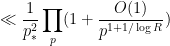
We may now eliminate the condition 


![\displaystyle \sum_{a_1,a_2 \in {\mathcal S}_J} \frac{k_0^{\Omega([a_1,a_2])}}{[a_1,a_2]} \sum_{d_1,d_2 \in {\mathcal S}_{I \cup J}: p_* | (d_1d_2,a_1a_2)}](https://s0.wp.com/latex.php?latex=%5Cdisplaystyle++%5Csum_%7Ba_1%2Ca_2+%5Cin+%7B%5Cmathcal+S%7D_J%7D+%5Cfrac%7Bk_0%5E%7B%5COmega%28%5Ba_1%2Ca_2%5D%29%7D%7D%7B%5Ba_1%2Ca_2%5D%7D+%5Csum_%7Bd_1%2Cd_2+%5Cin+%7B%5Cmathcal+S%7D_%7BI+%5Ccup+J%7D%3A+p_%2A+%7C+%28d_1d_2%2Ca_1a_2%29%7D&bg=ffffff&fg=000000&s=0&c=20201002)
![\displaystyle |g(\frac{\log a_1d_1}{\log R})| |g(\frac{\log a_1 d_2}{\log R})| \frac{k_0^{\Omega([d_1,d_2])}}{[d_1, d_2]}](https://s0.wp.com/latex.php?latex=%5Cdisplaystyle+%7Cg%28%5Cfrac%7B%5Clog+a_1d_1%7D%7B%5Clog+R%7D%29%7C+%7Cg%28%5Cfrac%7B%5Clog+a_1+d_2%7D%7B%5Clog+R%7D%29%7C+%5Cfrac%7Bk_0%5E%7B%5COmega%28%5Bd_1%2Cd_2%5D%29%7D%7D%7B%5Bd_1%2C+d_2%5D%7D&bg=ffffff&fg=000000&s=0&c=20201002)
can then be bounded by
![\displaystyle \ll \sum_{a_1,a_2} \sum_{d_1,d_2: p_* | (d_1d_2,a_1a_2)} \frac{k_0^{\Omega([a_1,a_2])}}{[a_1,a_2]} \frac{k_0^{\Omega([d_1,d_2])}}{[d_1, d_2]} (a_1 a_2 d_1 d_2)^{-1/\log R}](https://s0.wp.com/latex.php?latex=%5Cdisplaystyle++%5Cll+%5Csum_%7Ba_1%2Ca_2%7D+%5Csum_%7Bd_1%2Cd_2%3A+p_%2A+%7C+%28d_1d_2%2Ca_1a_2%29%7D+%5Cfrac%7Bk_0%5E%7B%5COmega%28%5Ba_1%2Ca_2%5D%29%7D%7D%7B%5Ba_1%2Ca_2%5D%7D+%5Cfrac%7Bk_0%5E%7B%5COmega%28%5Bd_1%2Cd_2%5D%29%7D%7D%7B%5Bd_1%2C+d_2%5D%7D+%28a_1+a_2+d_1+d_2%29%5E%7B-1%2F%5Clog+R%7D&bg=ffffff&fg=000000&s=0&c=20201002)
which may be factorised as
which by Mertens’ theorem (or the simple pole of 


Summing over all 
![\displaystyle \sum_{a_1,a_2 \in {\mathcal S}_J} \frac{\mu( (a_1,a_2) ) k_0^{\Omega([a_1,a_2])}}{[a_1,a_2]} \sum_{d_1,d_2\in {\mathcal S}_{I \cup J}}](https://s0.wp.com/latex.php?latex=%5Cdisplaystyle++%5Csum_%7Ba_1%2Ca_2+%5Cin+%7B%5Cmathcal+S%7D_J%7D+%5Cfrac%7B%5Cmu%28+%28a_1%2Ca_2%29+%29+k_0%5E%7B%5COmega%28%5Ba_1%2Ca_2%5D%29%7D%7D%7B%5Ba_1%2Ca_2%5D%7D+%5Csum_%7Bd_1%2Cd_2%5Cin+%7B%5Cmathcal+S%7D_%7BI+%5Ccup+J%7D%7D&bg=ffffff&fg=000000&s=0&c=20201002)
![\displaystyle \mu(d_1) g(\frac{\log a_1d_1}{\log R}) \mu(d_2) g(\frac{\log a_1 d_2}{\log R}) \frac{k_0^{\Omega([d_1,d_2])}}{[d_1, d_2]}.](https://s0.wp.com/latex.php?latex=%5Cdisplaystyle+%5Cmu%28d_1%29+g%28%5Cfrac%7B%5Clog+a_1d_1%7D%7B%5Clog+R%7D%29+%5Cmu%28d_2%29+g%28%5Cfrac%7B%5Clog+a_1+d_2%7D%7B%5Clog+R%7D%29+%5Cfrac%7Bk_0%5E%7B%5COmega%28%5Bd_1%2Cd_2%5D%29%7D%7D%7B%5Bd_1%2C+d_2%5D%7D.+&bg=ffffff&fg=000000&s=0&c=20201002)
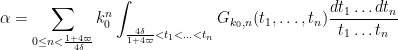
The inner summation can be treated using Proposition 10 of the previous post. We can then reduce (4) to
![\displaystyle \sum_{a_1,a_2 \in {\mathcal S}_J} \frac{\mu( (a_1,a_2) ) k_0^{\Omega([a_1,a_2])}}{[a_1,a_2]} G_{k_0}( \frac{\log a_1}{\log R}, \frac{\log a_2}{\log R} ) = \alpha+o(1) \ \ \ \ \ (7)](https://s0.wp.com/latex.php?latex=%5Cdisplaystyle++%5Csum_%7Ba_1%2Ca_2+%5Cin+%7B%5Cmathcal+S%7D_J%7D+%5Cfrac%7B%5Cmu%28+%28a_1%2Ca_2%29+%29+k_0%5E%7B%5COmega%28%5Ba_1%2Ca_2%5D%29%7D%7D%7B%5Ba_1%2Ca_2%5D%7D+G_%7Bk_0%7D%28+%5Cfrac%7B%5Clog+a_1%7D%7B%5Clog+R%7D%2C+%5Cfrac%7B%5Clog+a_2%7D%7B%5Clog+R%7D+%29+%3D+%5Calpha%2Bo%281%29+%5C+%5C+%5C+%5C+%5C+%287%29&bg=ffffff&fg=000000&s=0&c=20201002)
where 

Note that 


We rewrite the left-hand side of (7) as
![\displaystyle \sum_{a \in {\mathcal S}_J} \frac{k_0^{\Omega(a)}}{a} \sum_{a_1,a_2: [a_1,a_2] = a} \mu((a_1,a_2)) G_{k_0}( \frac{\log a_1}{\log R}, \frac{\log a_2}{\log R} ).](https://s0.wp.com/latex.php?latex=%5Cdisplaystyle++%5Csum_%7Ba+%5Cin+%7B%5Cmathcal+S%7D_J%7D+%5Cfrac%7Bk_0%5E%7B%5COmega%28a%29%7D%7D%7Ba%7D+%5Csum_%7Ba_1%2Ca_2%3A+%5Ba_1%2Ca_2%5D+%3D+a%7D+%5Cmu%28%28a_1%2Ca_2%29%29+G_%7Bk_0%7D%28+%5Cfrac%7B%5Clog+a_1%7D%7B%5Clog+R%7D%2C+%5Cfrac%7B%5Clog+a_2%7D%7B%5Clog+R%7D+%29.&bg=ffffff&fg=000000&s=0&c=20201002)
We may factor 


Using Mertens’ theorem, we thus conclude an exact formula for
Proposition 1 (Exact formula) We have
where
Similarly we have
where
are defined similarly to
by replacing all occurrences of
.


These formulae are unwieldy. However if we make some monotonicity hypotheses, namely that 


for 
![{t \in [0,1]}](https://s0.wp.com/latex.php?latex=%7Bt+%5Cin+%5B0%2C1%5D%7D&bg=ffffff&fg=000000&s=0&c=20201002)

for any 

for any 
and similarly

From Cauchy-Schwarz we thus have
Observe from the binomial formula that of the 


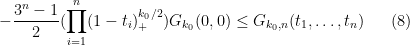
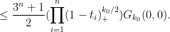
We have thus established the upper bound

where
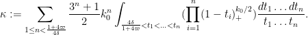
By symmetry we may factorise
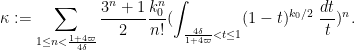
The expression 

and so

Note that


and hence

where

In practice we expect the 
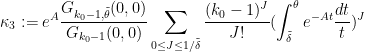
Now we turn to the estimation of


But we have an improvment in the lower bound in the

From the positive decreasing nature of 


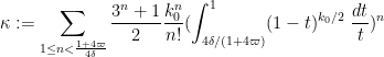
where
Estimating 

where

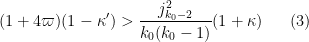
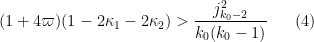
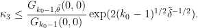
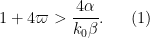
By (9), (10), we see that the condition (1) is implied by

By Theorem 14 and Lemma 15 of this previous post, we may take the ratio 

Theorem 2 Let
and
and suppose that
Then

As noted earlier, we heuristically have

and 

The purpose of this post is to isolate a combinatorial optimisation problem regarding subset sums; any improvement upon the current known bounds for this problem would lead to numerical improvements for the quantities pursued in the Polymath8 project. (UPDATE: Unfortunately no purely combinatorial improvement is possible, see comments.) We will also record the number-theoretic details of how this combinatorial problem is used in Zhang’s argument establishing bounded prime gaps.
First, some (rough) motivational background, omitting all the number-theoretic details and focusing on the combinatorics. (But readers who just want to see the combinatorial problem can skip the motivation and jump ahead to Lemma 5.) As part of the Polymath8 project we are trying to establish a certain estimate called 
Theorem 1 (Zhang’s theorem, numerically optimised)
.
Enlarging this region would lead to a better value of certain parameters 


I’ll state exactly what

for some bounded 


We can write 

A key technical feature of the Heath-Brown identity is that the weight 


The operation 


where 


Zhang’s argument splits into two major pieces, in which certain classes of (1) are established. Cheating a little bit, the following three results are established:
Theorem 2 (Type 0 estimate, informal version) The term (1) gives an acceptable contribution to
for some
.

Theorem 3 (Type I/II estimate, informal version) The term (1) gives an acceptable contribution to
where

Theorem 4 (Type III estimate, informal version) The term (1) gives an acceptable contribution to
with distinct
with
and


The above assertions are oversimplifications; there are some additional minor smallness hypotheses on
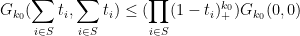
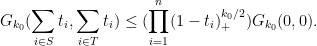
The deduction of Theorem 1 from Theorems 2, 3, 4 is then accomplished from the following, purely combinatorial, lemma:
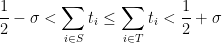
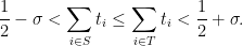
Lemma 5 (Subset sum lemma) Let
Let
Then at least one of the following statements hold:
- (Type 0) There is
such that
.
- (Type I/II) There is a partition
where
- (Type III) One can find distinct
and

The purely combinatorial question is whether the hypothesis (2) can be relaxed here to a weaker condition. This would allow us to improve the ranges for Theorem 1 (and hence for the values of
Let us review how this lemma is currently proven. The key sublemma is the following:
Lemma 6 Let
- (Type 0) There is a
.
- (Type I/II) There is a partition
- (Type III) There exist distinct
with
and
.
Proof: Suppose Type I/II never occurs, then every partial sum 


Call a summand 


By induction we see that if 


Now we see how Lemma 6 implies Lemma 5. Let

for some sufficiently small

and

with plenty of room to spare. We then apply Lemma 6. The Type 0 case of that lemma then implies the Type 0 case of Lemma 5, while the Type I/II case of Lemma 6 also implies the Type I/II case of Lemma 5. Finally, suppose that we are in the Type III case of Lemma 6. Since

we thus have
and so we will be done if
Inserting (3) and taking
but after some computation this is equivalent to (2).
It seems that there is some slack in this computation; some of the conclusions of the Type III case of Lemma 5, in particular, ended up being “wasted”, and it is possible that one did not fully exploit all the partial sums that could be used to create a Type I/II situation. So there may be a way to make improvements through purely combinatorial arguments. (UPDATE: As it turns out, this is sadly not the case: consderation of the case when 


A technical remark: for the application to Theorem 1, it is possible to enforce a bound on the number 


Below the fold I give the number-theoretic details of the combinatorial aspects of Zhang’s argument that correspond to the combinatorial problem described above.
This post is a continuation of the previous post on sieve theory, which is an ongoing part of the Polymath8 project to improve the various parameters in Zhang’s proof that bounded gaps between primes occur infinitely often. Given that the comments on that page are getting quite lengthy, this is also a good opportunity to “roll over” that thread.
We will continue the notation from the previous post, including the concept of an admissible tuple, the use of an asymptotic parameter
The objective of this portion of the Polymath8 project is to make as efficient as possible the connection between two types of results, which we call
Conjecture 1 (
Zhang was the first to prove a result of this type with 

There are two basic ways known currently to attain this conjecture. The first is to use the Elliott-Halberstam conjecture ![{EH[\theta]}](https://s0.wp.com/latex.php?latex=%7BEH%5B%5Ctheta%5D%7D&bg=ffffff&fg=000000&s=0&c=20201002)

Conjecture 2 (
for all fixed
for
.


Here of course 


In a breakthrough paper, Goldston, Yildirim, and Pintz established an implication of the form
![\displaystyle EH[\theta] \implies DHL[k_0,2] \ \ \ \ \ (1)](https://s0.wp.com/latex.php?latex=%5Cdisplaystyle++EH%5B%5Ctheta%5D+%5Cimplies+DHL%5Bk_0%2C2%5D+%5C+%5C+%5C+%5C+%5C+%281%29&bg=ffffff&fg=000000&s=0&c=20201002)
for any 


Theorem 3 (EH implies DHL) Let
where
is the first positive zero of the Bessel function
. Then
Note that the right-hand side of (2) is larger than 
Implications of the form Theorem 3 were modified by Motohashi and Pintz, which in our notation replaces
Conjecture 4 (
for any fixed
and
and


This is a weakened version of the Elliott-Halberstam conjecture:
Proposition 5 (EH implies MPZ) Let
implies
implies
In particular, since 
Proof: Define
then the hypothesis 

for any fixed
for any 


The contribution of the second term is 

and standard estimates we also have

and the claim now follows from the Cauchy-Schwarz inequality.
In practice, the conjecture ![{MPZ[\varpi,\varpi]}](https://s0.wp.com/latex.php?latex=%7BMPZ%5B%5Cvarpi%2C%5Cvarpi%5D%7D&bg=ffffff&fg=000000&s=0&c=20201002)


The work of Motohashi and Pintz, and later Zhang, implicitly describe arguments that allow one to deduce
Theorem 6 (MPZ implies DHL) Let
where
Then


This complicated version of 

We remark that as (5) is an open condition, it is unaffected by infinitesimal modifications to 
The known deductions of
Lemma 7 (Criterion for DHL) Let
is coprime to
, fixed quantities
, a quantity
for all
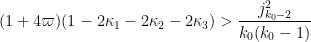
, and the key inequality
holds. Then
is defined to equal
when
otherwise.


By (6), (7), this quantity is at least

By (8), this expression is positive for all sufficiently large 


In practice, the quantity 


Once one has decided to rely on Lemma 7, the next main task is to select a good weight 
where 
for some weights 


One has a useful amount of flexibility in selecting the weights 

is used for some additional parameter 

for some suitable (in particular, sufficiently smooth) cutoff function
However, there is a slight variant choice of sieve weights that one can use, which I will call the “elementary Selberg sieve”, and it takes the form

for a sufficiently smooth function 
for 

for 

![\displaystyle \sum_{d_1,d_2 \in {\mathcal S}_I} \mu(d_1) a_{d_1} \mu(d_2) a_{d_2} \Delta([d_1,d_2])](https://s0.wp.com/latex.php?latex=%5Cdisplaystyle++%5Csum_%7Bd_1%2Cd_2+%5Cin+%7B%5Cmathcal+S%7D_I%7D+%5Cmu%28d_1%29+a_%7Bd_1%7D+%5Cmu%28d_2%29+a_%7Bd_2%7D+%5CDelta%28%5Bd_1%2Cd_2%5D%29&bg=ffffff&fg=000000&s=0&c=20201002)
(which arises naturally in the estimation of 
The use of the elementary Selberg sieve for the bounded prime gaps problem was studied by Motohashi and Pintz. Their arguments give an alternate derivation of ![{MPZ[\varpi,\theta]}](https://s0.wp.com/latex.php?latex=%7BMPZ%5B%5Cvarpi%2C%5Ctheta%5D%7D&bg=ffffff&fg=000000&s=0&c=20201002)

Below the fold we describe how the elementary Selberg sieve can be used to reprove Theorem 3, and discuss how they could potentially be used to improve upon Theorem 6. (But the elementary Selberg sieve and the analytic Selberg sieve are in any event closely related; see the appendix of this paper of mine with Ben Green for some further discussion.) For the purposes of polymath8, either developing the elementary Selberg sieve or continuing the analysis of the analytic Selberg sieve from the previous post would be a relevant topic of conversation in the comments to this post.

Recent Comments