
You are currently browsing the monthly archive for June 2019.
Let 


for any permutation 


will be an element of 


Given two natural numbers 

![{[F^{(k)}]_{k \rightarrow p} \in L(\Omega^p)_{sym}}](https://s0.wp.com/latex.php?latex=%7B%5BF%5E%7B%28k%29%7D%5D_%7Bk+%5Crightarrow+p%7D+%5Cin+L%28%5COmega%5Ep%29_%7Bsym%7D%7D&bg=ffffff&fg=000000&s=0&c=20201002)
![\displaystyle [F^{(k)}]_{k \rightarrow p}(x_1,\dots,x_p) = \sum_{1 \leq i_1 < i_2 < \dots < i_k \leq p} F^{(k)}(x_{i_1}, \dots, x_{i_k})](https://s0.wp.com/latex.php?latex=%5Cdisplaystyle+%5BF%5E%7B%28k%29%7D%5D_%7Bk+%5Crightarrow+p%7D%28x_1%2C%5Cdots%2Cx_p%29+%3D+%5Csum_%7B1+%5Cleq+i_1+%3C+i_2+%3C+%5Cdots+%3C+i_k+%5Cleq+p%7D+F%5E%7B%28k%29%7D%28x_%7Bi_1%7D%2C+%5Cdots%2C+x_%7Bi_k%7D%29+&bg=ffffff&fg=000000&s=0&c=20201002)
where 


![{[F^{(k)}]_{k \rightarrow p}}](https://s0.wp.com/latex.php?latex=%7B%5BF%5E%7B%28k%29%7D%5D_%7Bk+%5Crightarrow+p%7D%7D&bg=ffffff&fg=000000&s=0&c=20201002)
![\displaystyle [F^{(1)}(x_1)]_{1 \rightarrow p} = \sum_{i=1}^p F^{(1)}(x_i)](https://s0.wp.com/latex.php?latex=%5Cdisplaystyle+%5BF%5E%7B%281%29%7D%28x_1%29%5D_%7B1+%5Crightarrow+p%7D+%3D+%5Csum_%7Bi%3D1%7D%5Ep+F%5E%7B%281%29%7D%28x_i%29&bg=ffffff&fg=000000&s=0&c=20201002)
![\displaystyle [F^{(2)}(x_1,x_2)]_{2 \rightarrow p} = \sum_{1 \leq i < j \leq p} F^{(2)}(x_i,x_j)](https://s0.wp.com/latex.php?latex=%5Cdisplaystyle+%5BF%5E%7B%282%29%7D%28x_1%2Cx_2%29%5D_%7B2+%5Crightarrow+p%7D+%3D+%5Csum_%7B1+%5Cleq+i+%3C+j+%5Cleq+p%7D+F%5E%7B%282%29%7D%28x_i%2Cx_j%29&bg=ffffff&fg=000000&s=0&c=20201002)
and
![\displaystyle e_k^{(p)}(x_1,\dots,x_p) = [x_1 \dots x_k]_{k \rightarrow p}.](https://s0.wp.com/latex.php?latex=%5Cdisplaystyle+e_k%5E%7B%28p%29%7D%28x_1%2C%5Cdots%2Cx_p%29+%3D+%5Bx_1+%5Cdots+x_k%5D_%7Bk+%5Crightarrow+p%7D.&bg=ffffff&fg=000000&s=0&c=20201002)
Also we have
![\displaystyle [1]_{k \rightarrow p} = \binom{p}{k} = \frac{p(p-1)\dots(p-k+1)}{k!}.](https://s0.wp.com/latex.php?latex=%5Cdisplaystyle+%5B1%5D_%7Bk+%5Crightarrow+p%7D+%3D+%5Cbinom%7Bp%7D%7Bk%7D+%3D+%5Cfrac%7Bp%28p-1%29%5Cdots%28p-k%2B1%29%7D%7Bk%21%7D.&bg=ffffff&fg=000000&s=0&c=20201002)
With these conventions, we see that 


![\displaystyle [F^{(k)}]_{k \rightarrow p} = \frac{1}{\binom{p-k}{p-l}} [[F^{(k)}]_{k \rightarrow l}]_{l \rightarrow p}](https://s0.wp.com/latex.php?latex=%5Cdisplaystyle+%5BF%5E%7B%28k%29%7D%5D_%7Bk+%5Crightarrow+p%7D+%3D+%5Cfrac%7B1%7D%7B%5Cbinom%7Bp-k%7D%7Bp-l%7D%7D+%5B%5BF%5E%7B%28k%29%7D%5D_%7Bk+%5Crightarrow+l%7D%5D_%7Bl+%5Crightarrow+p%7D&bg=ffffff&fg=000000&s=0&c=20201002)
if 
The lifting map ![{[]_{k \rightarrow p}}](https://s0.wp.com/latex.php?latex=%7B%5B%5D_%7Bk+%5Crightarrow+p%7D%7D&bg=ffffff&fg=000000&s=0&c=20201002)


![\displaystyle [x_1]_{1 \rightarrow p} [x_1]_{1 \rightarrow p} = (\sum_{i=1}^p x_i)^2 \ \ \ \ \ (1)](https://s0.wp.com/latex.php?latex=%5Cdisplaystyle+%5Bx_1%5D_%7B1+%5Crightarrow+p%7D+%5Bx_1%5D_%7B1+%5Crightarrow+p%7D+%3D+%28%5Csum_%7Bi%3D1%7D%5Ep+x_i%29%5E2+%5C+%5C+%5C+%5C+%5C+%281%29&bg=ffffff&fg=000000&s=0&c=20201002)
![\displaystyle = [x_1^2]_{1 \rightarrow p} + 2 [x_1 x_2]_{1 \rightarrow p}](https://s0.wp.com/latex.php?latex=%5Cdisplaystyle+%3D+%5Bx_1%5E2%5D_%7B1+%5Crightarrow+p%7D+%2B+2+%5Bx_1+x_2%5D_%7B1+%5Crightarrow+p%7D&bg=ffffff&fg=000000&s=0&c=20201002)
![\displaystyle \neq [x_1^2]_{1 \rightarrow p}.](https://s0.wp.com/latex.php?latex=%5Cdisplaystyle+%5Cneq+%5Bx_1%5E2%5D_%7B1+%5Crightarrow+p%7D.&bg=ffffff&fg=000000&s=0&c=20201002)
In general, one has the identity
![\displaystyle [F^{(k)}(x_1,\dots,x_k)]_{k \rightarrow p} [G^{(l)}(x_1,\dots,x_l)]_{l \rightarrow p} = \sum_{k,l \leq m \leq k+l} \frac{1}{k! l!} \ \ \ \ \ (2)](https://s0.wp.com/latex.php?latex=%5Cdisplaystyle+%5BF%5E%7B%28k%29%7D%28x_1%2C%5Cdots%2Cx_k%29%5D_%7Bk+%5Crightarrow+p%7D+%5BG%5E%7B%28l%29%7D%28x_1%2C%5Cdots%2Cx_l%29%5D_%7Bl+%5Crightarrow+p%7D+%3D+%5Csum_%7Bk%2Cl+%5Cleq+m+%5Cleq+k%2Bl%7D+%5Cfrac%7B1%7D%7Bk%21+l%21%7D+%5C+%5C+%5C+%5C+%5C+%282%29&bg=ffffff&fg=000000&s=0&c=20201002)
![\displaystyle [\sum_{\pi, \rho} F^{(k)}(x_{\pi(1)},\dots,x_{\pi(k)}) G^{(l)}(x_{\rho(1)},\dots,x_{\rho(l)})]_{m \rightarrow p}](https://s0.wp.com/latex.php?latex=%5Cdisplaystyle+%5B%5Csum_%7B%5Cpi%2C+%5Crho%7D+F%5E%7B%28k%29%7D%28x_%7B%5Cpi%281%29%7D%2C%5Cdots%2Cx_%7B%5Cpi%28k%29%7D%29+G%5E%7B%28l%29%7D%28x_%7B%5Crho%281%29%7D%2C%5Cdots%2Cx_%7B%5Crho%28l%29%7D%29%5D_%7Bm+%5Crightarrow+p%7D&bg=ffffff&fg=000000&s=0&c=20201002)
for all natural numbers 


Example 1 When
, one has
which is just a restatement of the identity
![\displaystyle [x_1 x_2]_{2 \rightarrow p} [x_1]_{1 \rightarrow p} = [\frac{1}{2! 1!}( 2 x_1^2 x_2 + 2 x_1 x_2^2 )]_{2 \rightarrow p} + [\frac{1}{2! 1!} 6 x_1 x_2 x_3]_{3 \rightarrow p}](https://s0.wp.com/latex.php?latex=%5Cdisplaystyle+%5Bx_1+x_2%5D_%7B2+%5Crightarrow+p%7D+%5Bx_1%5D_%7B1+%5Crightarrow+p%7D+%3D+%5B%5Cfrac%7B1%7D%7B2%21+1%21%7D%28+2+x_1%5E2+x_2+%2B+2+x_1+x_2%5E2+%29%5D_%7B2+%5Crightarrow+p%7D+%2B+%5B%5Cfrac%7B1%7D%7B2%21+1%21%7D+6+x_1+x_2+x_3%5D_%7B3+%5Crightarrow+p%7D&bg=ffffff&fg=000000&s=0&c=20201002)
![\displaystyle = [x_1^2 x_2 + x_1 x_2^2]_{2 \rightarrow p} + [3x_1 x_2 x_3]_{3 \rightarrow p}](https://s0.wp.com/latex.php?latex=%5Cdisplaystyle+%3D+%5Bx_1%5E2+x_2+%2B+x_1+x_2%5E2%5D_%7B2+%5Crightarrow+p%7D+%2B+%5B3x_1+x_2+x_3%5D_%7B3+%5Crightarrow+p%7D&bg=ffffff&fg=000000&s=0&c=20201002)

Note that the coefficients appearing in (2) do not depend on the final number of variables 
![\displaystyle F^{(*)} = \sum_{k=0}^\infty [F^{(k)}]_{k \rightarrow *}](https://s0.wp.com/latex.php?latex=%5Cdisplaystyle+F%5E%7B%28%2A%29%7D+%3D+%5Csum_%7Bk%3D0%7D%5E%5Cinfty+%5BF%5E%7B%28k%29%7D%5D_%7Bk+%5Crightarrow+%2A%7D&bg=ffffff&fg=000000&s=0&c=20201002)
where for each 
![{[]_{k \rightarrow *}}](https://s0.wp.com/latex.php?latex=%7B%5B%5D_%7Bk+%5Crightarrow+%2A%7D%7D&bg=ffffff&fg=000000&s=0&c=20201002)
![\displaystyle [F^{(k)}]_{k \rightarrow *} + [G^{(k)}]_{k \rightarrow *} := [F^{(k)} + G^{(k)}]_{k \rightarrow *}](https://s0.wp.com/latex.php?latex=%5Cdisplaystyle+%5BF%5E%7B%28k%29%7D%5D_%7Bk+%5Crightarrow+%2A%7D+%2B+%5BG%5E%7B%28k%29%7D%5D_%7Bk+%5Crightarrow+%2A%7D+%3A%3D+%5BF%5E%7B%28k%29%7D+%2B+G%5E%7B%28k%29%7D%5D_%7Bk+%5Crightarrow+%2A%7D&bg=ffffff&fg=000000&s=0&c=20201002)
and
![\displaystyle c [F^{(k)}]_{k \rightarrow *} := [cF^{(k)}]_{k \rightarrow *}](https://s0.wp.com/latex.php?latex=%5Cdisplaystyle+c+%5BF%5E%7B%28k%29%7D%5D_%7Bk+%5Crightarrow+%2A%7D+%3A%3D+%5BcF%5E%7B%28k%29%7D%5D_%7Bk+%5Crightarrow+%2A%7D&bg=ffffff&fg=000000&s=0&c=20201002)
for 

![\displaystyle [F^{(k)}(x_1,\dots,x_k)]_{k \rightarrow *} [G^{(l)}(x_1,\dots,x_l)]_{l \rightarrow *} = \sum_{k,l \leq m \leq k+l} \frac{1}{k! l!} \ \ \ \ \ (3)](https://s0.wp.com/latex.php?latex=%5Cdisplaystyle+%5BF%5E%7B%28k%29%7D%28x_1%2C%5Cdots%2Cx_k%29%5D_%7Bk+%5Crightarrow+%2A%7D+%5BG%5E%7B%28l%29%7D%28x_1%2C%5Cdots%2Cx_l%29%5D_%7Bl+%5Crightarrow+%2A%7D+%3D+%5Csum_%7Bk%2Cl+%5Cleq+m+%5Cleq+k%2Bl%7D+%5Cfrac%7B1%7D%7Bk%21+l%21%7D+%5C+%5C+%5C+%5C+%5C+%283%29&bg=ffffff&fg=000000&s=0&c=20201002)
![\displaystyle [\sum_{\pi, \rho} F^{(k)}(x_{\pi(1)},\dots,x_{\pi(k)}) G^{(l)}(x_{\rho(1)},\dots,x_{\rho(l)})]_{m \rightarrow *}](https://s0.wp.com/latex.php?latex=%5Cdisplaystyle+%5B%5Csum_%7B%5Cpi%2C+%5Crho%7D+F%5E%7B%28k%29%7D%28x_%7B%5Cpi%281%29%7D%2C%5Cdots%2Cx_%7B%5Cpi%28k%29%7D%29+G%5E%7B%28l%29%7D%28x_%7B%5Crho%281%29%7D%2C%5Cdots%2Cx_%7B%5Crho%28l%29%7D%29%5D_%7Bm+%5Crightarrow+%2A%7D+&bg=ffffff&fg=000000&s=0&c=20201002)
of (2). Thus for instance, in this algebra
![\displaystyle [x_1]_{1 \rightarrow *} [x_1]_{1 \rightarrow *} = [x_1^2]_{1 \rightarrow *} + 2 [x_1 x_2]_{2 \rightarrow *}](https://s0.wp.com/latex.php?latex=%5Cdisplaystyle+%5Bx_1%5D_%7B1+%5Crightarrow+%2A%7D+%5Bx_1%5D_%7B1+%5Crightarrow+%2A%7D+%3D+%5Bx_1%5E2%5D_%7B1+%5Crightarrow+%2A%7D+%2B+2+%5Bx_1+x_2%5D_%7B2+%5Crightarrow+%2A%7D&bg=ffffff&fg=000000&s=0&c=20201002)
and
![\displaystyle [x_1 x_2]_{2 \rightarrow *} [x_1]_{1 \rightarrow *} = [x_1^2 x_2 + x_1 x_2^2]_{2 \rightarrow *} + [3 x_1 x_2 x_3]_{3 \rightarrow *}.](https://s0.wp.com/latex.php?latex=%5Cdisplaystyle+%5Bx_1+x_2%5D_%7B2+%5Crightarrow+%2A%7D+%5Bx_1%5D_%7B1+%5Crightarrow+%2A%7D+%3D+%5Bx_1%5E2+x_2+%2B+x_1+x_2%5E2%5D_%7B2+%5Crightarrow+%2A%7D+%2B+%5B3+x_1+x_2+x_3%5D_%7B3+%5Crightarrow+%2A%7D.&bg=ffffff&fg=000000&s=0&c=20201002)
Informally, ![{[1]_{0 \rightarrow *}}](https://s0.wp.com/latex.php?latex=%7B%5B1%5D_%7B0+%5Crightarrow+%2A%7D%7D&bg=ffffff&fg=000000&s=0&c=20201002)
For natural numbers ![{[]_{* \rightarrow p}}](https://s0.wp.com/latex.php?latex=%7B%5B%5D_%7B%2A+%5Crightarrow+p%7D%7D&bg=ffffff&fg=000000&s=0&c=20201002)
![\displaystyle [\sum_{k=0}^\infty [F^{(k)}]_{k \rightarrow *}]_{* \rightarrow p} := \sum_{k=0}^\infty [F^{(k)}]_{k \rightarrow p}.](https://s0.wp.com/latex.php?latex=%5Cdisplaystyle+%5B%5Csum_%7Bk%3D0%7D%5E%5Cinfty+%5BF%5E%7B%28k%29%7D%5D_%7Bk+%5Crightarrow+%2A%7D%5D_%7B%2A+%5Crightarrow+p%7D+%3A%3D+%5Csum_%7Bk%3D0%7D%5E%5Cinfty+%5BF%5E%7B%28k%29%7D%5D_%7Bk+%5Crightarrow+p%7D.&bg=ffffff&fg=000000&s=0&c=20201002)
Thus, for instance, ![{[x_1]_{1 \rightarrow *}}](https://s0.wp.com/latex.php?latex=%7B%5Bx_1%5D_%7B1+%5Crightarrow+%2A%7D%7D&bg=ffffff&fg=000000&s=0&c=20201002)
![{[x_1]_{1 \rightarrow p}}](https://s0.wp.com/latex.php?latex=%7B%5Bx_1%5D_%7B1+%5Crightarrow+p%7D%7D&bg=ffffff&fg=000000&s=0&c=20201002)
![{[x_1 x_2]_{2 \rightarrow *}}](https://s0.wp.com/latex.php?latex=%7B%5Bx_1+x_2%5D_%7B2+%5Crightarrow+%2A%7D%7D&bg=ffffff&fg=000000&s=0&c=20201002)
![{[x_1 x_2]_{2 \rightarrow p}}](https://s0.wp.com/latex.php?latex=%7B%5Bx_1+x_2%5D_%7B2+%5Crightarrow+p%7D%7D&bg=ffffff&fg=000000&s=0&c=20201002)
![{[]_{* \rightarrow p}: L(\Omega^*)_{sym} \rightarrow L(\Omega^p)_{sym}}](https://s0.wp.com/latex.php?latex=%7B%5B%5D_%7B%2A+%5Crightarrow+p%7D%3A+L%28%5COmega%5E%2A%29_%7Bsym%7D+%5Crightarrow+L%28%5COmega%5Ep%29_%7Bsym%7D%7D&bg=ffffff&fg=000000&s=0&c=20201002)
![{[]_{k \rightarrow *}: L(\Omega^k)_{sym} \rightarrow L(\Omega^*)_{sym}}](https://s0.wp.com/latex.php?latex=%7B%5B%5D_%7Bk+%5Crightarrow+%2A%7D%3A+L%28%5COmega%5Ek%29_%7Bsym%7D+%5Crightarrow+L%28%5COmega%5E%2A%29_%7Bsym%7D%7D&bg=ffffff&fg=000000&s=0&c=20201002)
![{[]_{k \rightarrow p}: L(\Omega^k)_{sym} \rightarrow L(\Omega^p)_{sym}}](https://s0.wp.com/latex.php?latex=%7B%5B%5D_%7Bk+%5Crightarrow+p%7D%3A+L%28%5COmega%5Ek%29_%7Bsym%7D+%5Crightarrow+L%28%5COmega%5Ep%29_%7Bsym%7D%7D&bg=ffffff&fg=000000&s=0&c=20201002)

Now suppose that we have a measure 


In the event that
![\displaystyle \int_{{\bf R}^p} [x_1]_{1 \rightarrow p}\ d\mu^p = p (\int_{\bf R} x\ d\mu(x)) (\int_{\bf R} \mu)^{p-1} \ \ \ \ \ (4)](https://s0.wp.com/latex.php?latex=%5Cdisplaystyle+%5Cint_%7B%7B%5Cbf+R%7D%5Ep%7D+%5Bx_1%5D_%7B1+%5Crightarrow+p%7D%5C+d%5Cmu%5Ep+%3D+p+%28%5Cint_%7B%5Cbf+R%7D+x%5C+d%5Cmu%28x%29%29+%28%5Cint_%7B%5Cbf+R%7D+%5Cmu%29%5E%7Bp-1%7D+%5C+%5C+%5C+%5C+%5C+%284%29&bg=ffffff&fg=000000&s=0&c=20201002)
![\displaystyle \int_{{\bf R}^p} [x_1 x_2]_{2 \rightarrow p}\ d\mu^p = \binom{p}{2} (\int_{{\bf R}^2} x_1 x_2\ d\mu(x_1) d\mu(x_2)) (\int_{\bf R} \mu)^{p-2}. \ \ \ \ \ (5)](https://s0.wp.com/latex.php?latex=%5Cdisplaystyle+%5Cint_%7B%7B%5Cbf+R%7D%5Ep%7D+%5Bx_1+x_2%5D_%7B2+%5Crightarrow+p%7D%5C+d%5Cmu%5Ep+%3D+%5Cbinom%7Bp%7D%7B2%7D+%28%5Cint_%7B%7B%5Cbf+R%7D%5E2%7D+x_1+x_2%5C+d%5Cmu%28x_1%29+d%5Cmu%28x_2%29%29+%28%5Cint_%7B%5Cbf+R%7D+%5Cmu%29%5E%7Bp-2%7D.+%5C+%5C+%5C+%5C+%5C+%285%29&bg=ffffff&fg=000000&s=0&c=20201002)
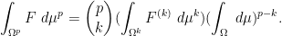
is an element of the formal algebra
![\displaystyle \int_{\Omega^p} [F^{(*)}]_{* \rightarrow p}\ d\mu^p = \sum_{k=0}^\infty \binom{p}{k} (\int_{\Omega^k} F^{(k)}\ d\mu^k) (\int_\Omega\ d\mu)^{p-k}. \ \ \ \ \ (6)](https://s0.wp.com/latex.php?latex=%5Cdisplaystyle+%5Cint_%7B%5COmega%5Ep%7D+%5BF%5E%7B%28%2A%29%7D%5D_%7B%2A+%5Crightarrow+p%7D%5C+d%5Cmu%5Ep+%3D+%5Csum_%7Bk%3D0%7D%5E%5Cinfty+%5Cbinom%7Bp%7D%7Bk%7D+%28%5Cint_%7B%5COmega%5Ek%7D+F%5E%7B%28k%29%7D%5C+d%5Cmu%5Ek%29+%28%5Cint_%5COmega%5C+d%5Cmu%29%5E%7Bp-k%7D.+%5C+%5C+%5C+%5C+%5C+%286%29&bg=ffffff&fg=000000&s=0&c=20201002)
Note that by hypothesis, only finitely many terms on the right-hand side are non-zero.
Now for a key observation: whereas the left-hand side of (6) only makes sense when 

![\displaystyle F^{(p)} = [F^{(*)}]_{* \rightarrow p} = \sum_{k=0}^\infty [F^{(k)}]_{k \rightarrow p}](https://s0.wp.com/latex.php?latex=%5Cdisplaystyle+F%5E%7B%28p%29%7D+%3D+%5BF%5E%7B%28%2A%29%7D%5D_%7B%2A+%5Crightarrow+p%7D+%3D+%5Csum_%7Bk%3D0%7D%5E%5Cinfty+%5BF%5E%7B%28k%29%7D%5D_%7Bk+%5Crightarrow+p%7D&bg=ffffff&fg=000000&s=0&c=20201002)
with 
![\displaystyle [F^{(*)}]_{* \rightarrow p} + [G^{(*)}]_{* \rightarrow p} := [F^{(*)} + G^{(*)}]_{* \rightarrow p}](https://s0.wp.com/latex.php?latex=%5Cdisplaystyle+%5BF%5E%7B%28%2A%29%7D%5D_%7B%2A+%5Crightarrow+p%7D+%2B+%5BG%5E%7B%28%2A%29%7D%5D_%7B%2A+%5Crightarrow+p%7D+%3A%3D+%5BF%5E%7B%28%2A%29%7D+%2B+G%5E%7B%28%2A%29%7D%5D_%7B%2A+%5Crightarrow+p%7D&bg=ffffff&fg=000000&s=0&c=20201002)
![\displaystyle c [F^{(*)}]_{* \rightarrow p} := [c F^{(*)}]_{* \rightarrow p}](https://s0.wp.com/latex.php?latex=%5Cdisplaystyle+c+%5BF%5E%7B%28%2A%29%7D%5D_%7B%2A+%5Crightarrow+p%7D+%3A%3D+%5Bc+F%5E%7B%28%2A%29%7D%5D_%7B%2A+%5Crightarrow+p%7D&bg=ffffff&fg=000000&s=0&c=20201002)
![\displaystyle [F^{(*)}]_{* \rightarrow p} [G^{(*)}]_{* \rightarrow p} := [F^{(*)} G^{(*)}]_{* \rightarrow p}.](https://s0.wp.com/latex.php?latex=%5Cdisplaystyle+%5BF%5E%7B%28%2A%29%7D%5D_%7B%2A+%5Crightarrow+p%7D+%5BG%5E%7B%28%2A%29%7D%5D_%7B%2A+%5Crightarrow+p%7D+%3A%3D+%5BF%5E%7B%28%2A%29%7D+G%5E%7B%28%2A%29%7D%5D_%7B%2A+%5Crightarrow+p%7D.&bg=ffffff&fg=000000&s=0&c=20201002)
In particular, the multiplication law (2) continues to hold for such values of 

Example 2 Suppose
is a random variable; on any power
, we let
be the usual independent copies of
on
for
. Then for any real or complex
can be evaluated by first using the identity
(cf. (1)) and then using (6) and the probability measure hypothesis
to conclude that
For
whenever
are jointly independent copies of
has expectation
and variance
. One can thus view (7) as an abstract generalisation of (8) to the case when
In this particular case, the quantity (7) is non-negative for every nonnegative
and the right-hand side can become negative for
. This is a shame, because otherwise one could hope to start endowing
with some sort of commutative von Neumann algebra type structure (or the abstract probability structure discussed in this previous post) and then interpret it as a genuine measure space rather than as a virtual one. (This failure of positivity is related to the fact that the characteristic function of a random variable, when raised to the
is non-negative, then so is
![\displaystyle \int_{\Omega^p} [X_1]_{1 \rightarrow p}^2\ d\mu^p](https://s0.wp.com/latex.php?latex=%5Cdisplaystyle+%5Cint_%7B%5COmega%5Ep%7D+%5BX_1%5D_%7B1+%5Crightarrow+p%7D%5E2%5C+d%5Cmu%5Ep+&bg=ffffff&fg=000000&s=0&c=20201002)
![\displaystyle [X_1]_{1 \rightarrow p}^2 = [X_1^2]_{1 \rightarrow p} + 2[X_1 X_2]_{2 \rightarrow p}](https://s0.wp.com/latex.php?latex=%5Cdisplaystyle+%5BX_1%5D_%7B1+%5Crightarrow+p%7D%5E2+%3D+%5BX_1%5E2%5D_%7B1+%5Crightarrow+p%7D+%2B+2%5BX_1+X_2%5D_%7B2+%5Crightarrow+p%7D&bg=ffffff&fg=000000&s=0&c=20201002)
![\displaystyle \int_{\Omega^p} [X_1]_{1 \rightarrow p}^2\ d\mu^p = \binom{p}{1} \int_{\Omega} X^2\ d\mu + 2 \binom{p}{2} \int_{\Omega^2} X_1 X_2\ d\mu^2](https://s0.wp.com/latex.php?latex=%5Cdisplaystyle+%5Cint_%7B%5COmega%5Ep%7D+%5BX_1%5D_%7B1+%5Crightarrow+p%7D%5E2%5C+d%5Cmu%5Ep+%3D+%5Cbinom%7Bp%7D%7B1%7D+%5Cint_%7B%5COmega%7D+X%5E2%5C+d%5Cmu+%2B+2+%5Cbinom%7Bp%7D%7B2%7D+%5Cint_%7B%5COmega%5E2%7D+X_1+X_2%5C+d%5Cmu%5E2&bg=ffffff&fg=000000&s=0&c=20201002)

![\displaystyle \int_{\Omega^p} [X_1]_{1 \rightarrow p}^2\ d\mu^p = p \mathbf{Var}(X) + p^2 \mathbf{E}(X)^2. \ \ \ \ \ (7)](https://s0.wp.com/latex.php?latex=%5Cdisplaystyle+%5Cint_%7B%5COmega%5Ep%7D+%5BX_1%5D_%7B1+%5Crightarrow+p%7D%5E2%5C+d%5Cmu%5Ep+%3D+p+%5Cmathbf%7BVar%7D%28X%29+%2B+p%5E2+%5Cmathbf%7BE%7D%28X%29%5E2.+%5C+%5C+%5C+%5C+%5C+%287%29&bg=ffffff&fg=000000&s=0&c=20201002)

![\displaystyle \int_{\Omega^p} [X_1]_{1 \rightarrow p}^4\ d\mu^p = p \mathbf{Var}(X^2) + p(3p-2) (\mathbf{E}(X^2))^2](https://s0.wp.com/latex.php?latex=%5Cdisplaystyle+%5Cint_%7B%5COmega%5Ep%7D+%5BX_1%5D_%7B1+%5Crightarrow+p%7D%5E4%5C+d%5Cmu%5Ep+%3D+p+%5Cmathbf%7BVar%7D%28X%5E2%29+%2B+p%283p-2%29+%28%5Cmathbf%7BE%7D%28X%5E2%29%29%5E2&bg=ffffff&fg=000000&s=0&c=20201002)
![\displaystyle \int_{\Omega^p} [F]_{1 \rightarrow p}\ d\mu^p = p (\int_\Omega F\ d\mu) (\int_\Omega\ d\mu)^{p-1}.](https://s0.wp.com/latex.php?latex=%5Cdisplaystyle+%5Cint_%7B%5COmega%5Ep%7D+%5BF%5D_%7B1+%5Crightarrow+p%7D%5C+d%5Cmu%5Ep+%3D+p+%28%5Cint_%5COmega+F%5C+d%5Cmu%29+%28%5Cint_%5COmega%5C+d%5Cmu%29%5E%7Bp-1%7D.&bg=ffffff&fg=000000&s=0&c=20201002)
One can wonder what the point is to all of this abstract formalism and how it relates to the rest of mathematics. For me, this formalism originated implicitly in an old paper I wrote with Jon Bennett and Tony Carbery on the multilinear restriction and Kakeya conjectures, though we did not have a good language for working with it at the time, instead working first with the case of natural number exponents

(where the right-hand side should be viewed as the fractional dimensional integral of the unit ![{[1]_{0 \rightarrow p}}](https://s0.wp.com/latex.php?latex=%7B%5B1%5D_%7B0+%5Crightarrow+p%7D%7D&bg=ffffff&fg=000000&s=0&c=20201002)
Lemma 3 (Differentiation formula) Suppose that a positive measure
on
and varies by the formula
for some function
. Let
for all
that are independent of
to now depend on
again assuming sufficient amounts of smoothness and regularity.

![\displaystyle \frac{d}{dt} \int_{\Omega^p} F^{(p)}\ d\mu(t)^p = \int_{\Omega^p} F^{(p)} [a(t)]_{1 \rightarrow p}\ d\mu(t)^p \ \ \ \ \ (10)](https://s0.wp.com/latex.php?latex=%5Cdisplaystyle+%5Cfrac%7Bd%7D%7Bdt%7D+%5Cint_%7B%5COmega%5Ep%7D+F%5E%7B%28p%29%7D%5C+d%5Cmu%28t%29%5Ep+%3D+%5Cint_%7B%5COmega%5Ep%7D+F%5E%7B%28p%29%7D+%5Ba%28t%29%5D_%7B1+%5Crightarrow+p%7D%5C+d%5Cmu%28t%29%5Ep+%5C+%5C+%5C+%5C+%5C+%2810%29&bg=ffffff&fg=000000&s=0&c=20201002)

![\displaystyle = \int_{\Omega^p} \frac{d}{dt} F^{(p)}(t) + F^{(p)}(t) [a(t)]_{1 \rightarrow p}\ d\mu(t)^p,](https://s0.wp.com/latex.php?latex=%5Cdisplaystyle+%3D+%5Cint_%7B%5COmega%5Ep%7D+%5Cfrac%7Bd%7D%7Bdt%7D+F%5E%7B%28p%29%7D%28t%29+%2B+F%5E%7B%28p%29%7D%28t%29+%5Ba%28t%29%5D_%7B1+%5Crightarrow+p%7D%5C+d%5Cmu%28t%29%5Ep%2C+&bg=ffffff&fg=000000&s=0&c=20201002)
Proof: We just prove (10), as (11) then follows by same argument used to prove the usual product rule. By linearity it suffices to verify this identity in the case ![{F^{(p)} = [F^{(k)}]_{k \rightarrow p}}](https://s0.wp.com/latex.php?latex=%7BF%5E%7B%28p%29%7D+%3D+%5BF%5E%7B%28k%29%7D%5D_%7Bk+%5Crightarrow+p%7D%7D&bg=ffffff&fg=000000&s=0&c=20201002)
![\displaystyle \frac{d}{dt} [\binom{p}{k} (\int_{\Omega^k} F^{(k)}\ d\mu(t)^k) (\int_\Omega\ d\mu(t))^{p-k}]. \ \ \ \ \ (12)](https://s0.wp.com/latex.php?latex=%5Cdisplaystyle+%5Cfrac%7Bd%7D%7Bdt%7D+%5B%5Cbinom%7Bp%7D%7Bk%7D+%28%5Cint_%7B%5COmega%5Ek%7D+F%5E%7B%28k%29%7D%5C+d%5Cmu%28t%29%5Ek%29+%28%5Cint_%5COmega%5C+d%5Cmu%28t%29%29%5E%7Bp-k%7D%5D.+%5C+%5C+%5C+%5C+%5C+%2812%29&bg=ffffff&fg=000000&s=0&c=20201002)
Differentiating under the integral sign using (9) we have
and similarly

where 

By the product rule, we can thus expand (12) as
where we have suppressed the dependence on 
![\displaystyle \int_{\Omega^p} [F^{(k)} (a_1 + \dots + a_k)]_{k \rightarrow p} + [ F^{(k)} \ast a ]_{k+1 \rightarrow p}\ d\mu^p](https://s0.wp.com/latex.php?latex=%5Cdisplaystyle+%5Cint_%7B%5COmega%5Ep%7D+%5BF%5E%7B%28k%29%7D+%28a_1+%2B+%5Cdots+%2B+a_k%29%5D_%7Bk+%5Crightarrow+p%7D+%2B+%5B+F%5E%7B%28k%29%7D+%5Cast+a+%5D_%7Bk%2B1+%5Crightarrow+p%7D%5C+d%5Cmu%5Ep&bg=ffffff&fg=000000&s=0&c=20201002)
where 

But from (2) one has
![\displaystyle [F^{(k)} (a_1 + \dots + a_k)]_{k \rightarrow p} + [ F^{(k)} \ast a ]_{k+1 \rightarrow p} = [F^{(k)}]_{k \rightarrow p} [a]_{1 \rightarrow p}](https://s0.wp.com/latex.php?latex=%5Cdisplaystyle+%5BF%5E%7B%28k%29%7D+%28a_1+%2B+%5Cdots+%2B+a_k%29%5D_%7Bk+%5Crightarrow+p%7D+%2B+%5B+F%5E%7B%28k%29%7D+%5Cast+a+%5D_%7Bk%2B1+%5Crightarrow+p%7D+%3D+%5BF%5E%7B%28k%29%7D%5D_%7Bk+%5Crightarrow+p%7D+%5Ba%5D_%7B1+%5Crightarrow+p%7D&bg=ffffff&fg=000000&s=0&c=20201002)
and the claim follows.

Remark 4 It is also instructive to prove this lemma in the special case when
can be interpreted as a classical integral. In this case, the identity (10) is immediate from applying the product rule to (9) to conclude that
One could in fact derive (10) for arbitrary real or complex
![\displaystyle \frac{d}{dt} d\mu(t)^p = [a(t)]_{1 \rightarrow p} d\mu(t)^p.](https://s0.wp.com/latex.php?latex=%5Cdisplaystyle+%5Cfrac%7Bd%7D%7Bdt%7D+d%5Cmu%28t%29%5Ep+%3D+%5Ba%28t%29%5D_%7B1+%5Crightarrow+p%7D+d%5Cmu%28t%29%5Ep.&bg=ffffff&fg=000000&s=0&c=20201002)
Let us give a simple PDE application of this lemma as illustration:
Proposition 5 (Heat flow monotonicity) Let
be a solution to the heat equation
with initial data
a rapidly decreasing finite non-negative Radon measure, or more explicitly
for al
. Then for any
, the quantity
is monotone non-decreasing in
for
, constant for
, and monotone non-increasing for
.


Proof: By a limiting argument we may assume that 
For any 

Then the quantity 
Observe that

and thus by Lemma 3 and the product rule
![\displaystyle \frac{d}{dt} Q_p(t) = -\frac{d}{2t} Q_p(t) + t^{-d/2} \int_{{\bf R}^d} \int_{({\bf R}^d)^p} [\frac{|x-y|^2}{4t^2}]_{1 \rightarrow p} d\mu(t,x)^p\ dx \ \ \ \ \ (13)](https://s0.wp.com/latex.php?latex=%5Cdisplaystyle+%5Cfrac%7Bd%7D%7Bdt%7D+Q_p%28t%29+%3D+-%5Cfrac%7Bd%7D%7B2t%7D+Q_p%28t%29+%2B+t%5E%7B-d%2F2%7D+%5Cint_%7B%7B%5Cbf+R%7D%5Ed%7D+%5Cint_%7B%28%7B%5Cbf+R%7D%5Ed%29%5Ep%7D+%5B%5Cfrac%7B%7Cx-y%7C%5E2%7D%7B4t%5E2%7D%5D_%7B1+%5Crightarrow+p%7D+d%5Cmu%28t%2Cx%29%5Ep%5C+dx+%5C+%5C+%5C+%5C+%5C+%2813%29&bg=ffffff&fg=000000&s=0&c=20201002)
where we use 


To simplify this expression we will take advantage of integration by parts in the 

and hence by Lemma 3
![\displaystyle \frac{\partial}{\partial x_j} \int_{({\bf R}^d)^p}\ d\mu(t,x)^p\ dx = - \int_{({\bf R}^d)^p} [\frac{x_j-y_j}{2t}]_{1 \rightarrow p}\ d\mu(t,x)^p\ dx.](https://s0.wp.com/latex.php?latex=%5Cdisplaystyle+%5Cfrac%7B%5Cpartial%7D%7B%5Cpartial+x_j%7D+%5Cint_%7B%28%7B%5Cbf+R%7D%5Ed%29%5Ep%7D%5C+d%5Cmu%28t%2Cx%29%5Ep%5C+dx+%3D+-+%5Cint_%7B%28%7B%5Cbf+R%7D%5Ed%29%5Ep%7D+%5B%5Cfrac%7Bx_j-y_j%7D%7B2t%7D%5D_%7B1+%5Crightarrow+p%7D%5C+d%5Cmu%28t%2Cx%29%5Ep%5C+dx.&bg=ffffff&fg=000000&s=0&c=20201002)
Multiplying by
![\displaystyle d Q_p(t) = \int_{{\bf R}^d} \int_{({\bf R}^d)^p} x_j [\frac{x_j-y_j}{2t}]_{1 \rightarrow p}\ d\mu(t,x)^p\ dx](https://s0.wp.com/latex.php?latex=%5Cdisplaystyle+d+Q_p%28t%29+%3D+%5Cint_%7B%7B%5Cbf+R%7D%5Ed%7D+%5Cint_%7B%28%7B%5Cbf+R%7D%5Ed%29%5Ep%7D+x_j+%5B%5Cfrac%7Bx_j-y_j%7D%7B2t%7D%5D_%7B1+%5Crightarrow+p%7D%5C+d%5Cmu%28t%2Cx%29%5Ep%5C+dx&bg=ffffff&fg=000000&s=0&c=20201002)
![\displaystyle = \int_{{\bf R}^d} \int_{({\bf R}^d)^p} x_j [\frac{x_j-y_j}{2t}]_{1 \rightarrow p}\ d\mu(t,x)^p\ dx](https://s0.wp.com/latex.php?latex=%5Cdisplaystyle+%3D+%5Cint_%7B%7B%5Cbf+R%7D%5Ed%7D+%5Cint_%7B%28%7B%5Cbf+R%7D%5Ed%29%5Ep%7D+x_j+%5B%5Cfrac%7Bx_j-y_j%7D%7B2t%7D%5D_%7B1+%5Crightarrow+p%7D%5C+d%5Cmu%28t%2Cx%29%5Ep%5C+dx&bg=ffffff&fg=000000&s=0&c=20201002)
where we use the Einstein summation convention in 

![\displaystyle \frac{\partial}{\partial x_j} \int_{({\bf R}^d)^p}[F_j(y)]_{1 \rightarrow p}\ d\mu(t,x)^p\ dx](https://s0.wp.com/latex.php?latex=%5Cdisplaystyle+%5Cfrac%7B%5Cpartial%7D%7B%5Cpartial+x_j%7D+%5Cint_%7B%28%7B%5Cbf+R%7D%5Ed%29%5Ep%7D%5BF_j%28y%29%5D_%7B1+%5Crightarrow+p%7D%5C+d%5Cmu%28t%2Cx%29%5Ep%5C+dx+&bg=ffffff&fg=000000&s=0&c=20201002)
![\displaystyle = - \int_{({\bf R}^d)^p} [F_j(y)]_{1 \rightarrow p} [\frac{x_j-y_j}{2t}]_{1 \rightarrow p}\ d\mu(t,x)^p\ dx](https://s0.wp.com/latex.php?latex=%5Cdisplaystyle+%3D+-+%5Cint_%7B%28%7B%5Cbf+R%7D%5Ed%29%5Ep%7D+%5BF_j%28y%29%5D_%7B1+%5Crightarrow+p%7D+%5B%5Cfrac%7Bx_j-y_j%7D%7B2t%7D%5D_%7B1+%5Crightarrow+p%7D%5C+d%5Cmu%28t%2Cx%29%5Ep%5C+dx&bg=ffffff&fg=000000&s=0&c=20201002)
and hence on integration by parts
![\displaystyle 0 = \int_{{\bf R}^d} \int_{({\bf R}^d)^p} [F_j(y) \frac{x_j-y_j}{2t}]_{1 \rightarrow p}\ d\mu(t,x)^p\ dx.](https://s0.wp.com/latex.php?latex=%5Cdisplaystyle+0+%3D+%5Cint_%7B%7B%5Cbf+R%7D%5Ed%7D+%5Cint_%7B%28%7B%5Cbf+R%7D%5Ed%29%5Ep%7D+%5BF_j%28y%29+%5Cfrac%7Bx_j-y_j%7D%7B2t%7D%5D_%7B1+%5Crightarrow+p%7D%5C+d%5Cmu%28t%2Cx%29%5Ep%5C+dx.&bg=ffffff&fg=000000&s=0&c=20201002)
We conclude that
![\displaystyle \frac{d}{2t} Q_p(t) = t^{-d/2} \int_{{\bf R}^d} \int_{({\bf R}^d)^p} (x_j - [F_j(y)]_{1 \rightarrow p}) [\frac{(x_j-y_j)}{4t}]_{1 \rightarrow p} d\mu(t,x)^p\ dx](https://s0.wp.com/latex.php?latex=%5Cdisplaystyle+%5Cfrac%7Bd%7D%7B2t%7D+Q_p%28t%29+%3D+t%5E%7B-d%2F2%7D+%5Cint_%7B%7B%5Cbf+R%7D%5Ed%7D+%5Cint_%7B%28%7B%5Cbf+R%7D%5Ed%29%5Ep%7D+%28x_j+-+%5BF_j%28y%29%5D_%7B1+%5Crightarrow+p%7D%29+%5B%5Cfrac%7B%28x_j-y_j%29%7D%7B4t%7D%5D_%7B1+%5Crightarrow+p%7D+d%5Cmu%28t%2Cx%29%5Ep%5C+dx+&bg=ffffff&fg=000000&s=0&c=20201002)
and thus by (13)
![\displaystyle [(x_j-y_j)(x_j-y_j)]_{1 \rightarrow p} - (x_j - [F_j(y)]_{1 \rightarrow p}) [x_j - y_j]_{1 \rightarrow p}\ d\mu(t,x)^p\ dx.](https://s0.wp.com/latex.php?latex=%5Cdisplaystyle+%5B%28x_j-y_j%29%28x_j-y_j%29%5D_%7B1+%5Crightarrow+p%7D+-+%28x_j+-+%5BF_j%28y%29%5D_%7B1+%5Crightarrow+p%7D%29+%5Bx_j+-+y_j%5D_%7B1+%5Crightarrow+p%7D%5C+d%5Cmu%28t%2Cx%29%5Ep%5C+dx.&bg=ffffff&fg=000000&s=0&c=20201002)
The choice of 

![{x_j - [F_j(y)]_{1 \rightarrow p} = \frac{1}{p} [x_j - y_j]_{1 \rightarrow p}}](https://s0.wp.com/latex.php?latex=%7Bx_j+-+%5BF_j%28y%29%5D_%7B1+%5Crightarrow+p%7D+%3D+%5Cfrac%7B1%7D%7Bp%7D+%5Bx_j+-+y_j%5D_%7B1+%5Crightarrow+p%7D%7D&bg=ffffff&fg=000000&s=0&c=20201002)
![\displaystyle \int_{({\bf R}^d)^p} [(x_j-y_j)(x_j-y_j)]_{1 \rightarrow p}\ d\mu^p = p \mathop{\bf E} |x-Y|^2 (\int_{{\bf R}^d}\ d\mu)^{p}](https://s0.wp.com/latex.php?latex=%5Cdisplaystyle+%5Cint_%7B%28%7B%5Cbf+R%7D%5Ed%29%5Ep%7D+%5B%28x_j-y_j%29%28x_j-y_j%29%5D_%7B1+%5Crightarrow+p%7D%5C+d%5Cmu%5Ep+%3D+p+%5Cmathop%7B%5Cbf+E%7D+%7Cx-Y%7C%5E2+%28%5Cint_%7B%7B%5Cbf+R%7D%5Ed%7D%5C+d%5Cmu%29%5E%7Bp%7D&bg=ffffff&fg=000000&s=0&c=20201002)
and
![\displaystyle \int_{({\bf R}^d)^p} [x_j-y_j]_{1 \rightarrow p} [x_j-y_j]_{1 \rightarrow p}\ d\mu^p](https://s0.wp.com/latex.php?latex=%5Cdisplaystyle+%5Cint_%7B%28%7B%5Cbf+R%7D%5Ed%29%5Ep%7D+%5Bx_j-y_j%5D_%7B1+%5Crightarrow+p%7D+%5Bx_j-y_j%5D_%7B1+%5Crightarrow+p%7D%5C+d%5Cmu%5Ep+&bg=ffffff&fg=000000&s=0&c=20201002)

where 


This expression is clearly non-negative for 


Remark 6 As with Remark 4, one can also establish the identity (14) first for natural numbers
A more complicated version of this argument establishes the non-endpoint multilinear Kakeya inequality (without any logarithmic loss in a scale parameter 
The AMS and MAA have recently published (and made available online) a collection of essays entitled “Living Proof: Stories of Resilience Along the Mathematical Journey”. Each author contributes a story of how they encountered some internal or external difficulty in advancing their mathematical career, and how they were able to deal with such difficulties. I myself have contributed one of these essays; I was initially somewhat surprised when I was approached for a contribution, as my career trajectory has been somewhat of an outlier, and I have been very fortunate to not experience to the same extent many of the obstacles that other contributors write about in this text. Nevertheless there was a turning point in my career that I write about here during my graduate years, when I found that the improvised and poorly disciplined study habits that were able to get me into graduate school due to an over-reliance on raw mathematical ability were completely inadequate to handle the graduate qualifying exam. With a combination of an astute advisor and some sheer luck, I was able to pass the exam and finally develop a more sustainable approach to learning and doing mathematics, but it could easily have gone quite differently. (My 20 25-year old writeup of this examination, complete with spelling errors, may be found here.)
The following situation is very common in modern harmonic analysis: one has a large scale parameter 


for all 
for all 


in which case the property of having a subpolynomial upper bound is equivalent to that of being subpolynomial size in the sense that

for all
Let us give some illustrative examples of this type of problem:
Example 1 (Kakeya conjecture) Here
be a fixed dimension. For each
, we pick a maximal
-separated set of directions
. We let
where
is a
-tube oriented in the direction
. The Kakeya maximal function conjecture is then equivalent to the assertion that
.
Example 2 (Restriction conjecture for the sphere) Here
for all bounded measurable functions
on the unit sphere
equipped with surface measure
, where
is the ball of radius

Example 3 (Multilinear Kakeya inequality) Again
be compact subsets of the sphere
for the wedge product of directions
for
(equivalently, there is no hyperplane through the origin that intersects all of the
). For each
where for each
is a collection of infinite tubes in
oriented in a direction in
in
is our notation for the geometric mean
The multilinear Kakeya inequality of Bennett, Carbery, and myself establishes that
Example 4 (Multilinear restriction theorem) Once again
for all bounded measurable functions
on
.
Example 5 (Decoupling for the paraboloid)
into
cubes
of sidelength
. For any
, define the extension operators
and
for
and
. We also introduce the weight function
For any
be the smallest constant for which one has the decoupling inequality
The decoupling theorem of Bourgain and Demeter asserts that
.
![\displaystyle E_{[0,1]^{d-1}} g( x', x_d ) := \int_{[0,1]^{d-1}} e^{2\pi i (x' \cdot \xi + x_d |\xi|^2)} g(\xi)\ d\xi](https://s0.wp.com/latex.php?latex=%5Cdisplaystyle++E_%7B%5B0%2C1%5D%5E%7Bd-1%7D%7D+g%28+x%27%2C+x_d+%29+%3A%3D+%5Cint_%7B%5B0%2C1%5D%5E%7Bd-1%7D%7D+e%5E%7B2%5Cpi+i+%28x%27+%5Ccdot+%5Cxi+%2B+x_d+%7C%5Cxi%7C%5E2%29%7D+g%28%5Cxi%29%5C+d%5Cxi&bg=ffffff&fg=000000&s=0&c=20201002)
![\displaystyle \| E_{[0,1]^{d-1}} g \|_{L^p(w_{B(0,N)})} \leq D_p(N) (\sum_Q \| E_Q g \|_{L^p(w_{B(0,N)})}^2)^{1/2}.](https://s0.wp.com/latex.php?latex=%5Cdisplaystyle++%5C%7C+E_%7B%5B0%2C1%5D%5E%7Bd-1%7D%7D+g+%5C%7C_%7BL%5Ep%28w_%7BB%280%2CN%29%7D%29%7D+%5Cleq+D_p%28N%29+%28%5Csum_Q+%5C%7C+E_Q+g+%5C%7C_%7BL%5Ep%28w_%7BB%280%2CN%29%7D%29%7D%5E2%29%5E%7B1%2F2%7D.&bg=ffffff&fg=000000&s=0&c=20201002)
Example 6 (Decoupling for the moment curve)
into
of length
, define the extension operators
and more generally
for
. For any
It was shown by Bourgain, Demeter, and Guth that
, which among other things implies the Vinogradov main conjecture (as discussed in this previous post).
![\displaystyle E_{[0,1]} g(x_1,\dots,x_d) = \int_{[0,1]} e^{2\pi i ( x_1 \xi + x_2 \xi^2 + \dots + x_d \xi^d} g(\xi)\ d\xi](https://s0.wp.com/latex.php?latex=%5Cdisplaystyle++E_%7B%5B0%2C1%5D%7D+g%28x_1%2C%5Cdots%2Cx_d%29+%3D+%5Cint_%7B%5B0%2C1%5D%7D+e%5E%7B2%5Cpi+i+%28+x_1+%5Cxi+%2B+x_2+%5Cxi%5E2+%2B+%5Cdots+%2B+x_d+%5Cxi%5Ed%7D+g%28%5Cxi%29%5C+d%5Cxi&bg=ffffff&fg=000000&s=0&c=20201002)
![\displaystyle E_J g(x_1,\dots,x_d) = \int_{[0,1]} e^{2\pi i ( x_1 \xi + x_2 \xi^2 + \dots + x_d \xi^d} g(\xi)\ d\xi](https://s0.wp.com/latex.php?latex=%5Cdisplaystyle++E_J+g%28x_1%2C%5Cdots%2Cx_d%29+%3D+%5Cint_%7B%5B0%2C1%5D%7D+e%5E%7B2%5Cpi+i+%28+x_1+%5Cxi+%2B+x_2+%5Cxi%5E2+%2B+%5Cdots+%2B+x_d+%5Cxi%5Ed%7D+g%28%5Cxi%29%5C+d%5Cxi&bg=ffffff&fg=000000&s=0&c=20201002)
![\displaystyle \| E_{[0,1]} g \|_{L^p(w_{B(0,N^d)})} \leq D_p(N) (\sum_J \| E_J g \|_{L^p(w_{B(0,N^d)})}^2)^{1/2}.](https://s0.wp.com/latex.php?latex=%5Cdisplaystyle++%5C%7C+E_%7B%5B0%2C1%5D%7D+g+%5C%7C_%7BL%5Ep%28w_%7BB%280%2CN%5Ed%29%7D%29%7D+%5Cleq+D_p%28N%29+%28%5Csum_J+%5C%7C+E_J+g+%5C%7C_%7BL%5Ep%28w_%7BB%280%2CN%5Ed%29%7D%29%7D%5E2%29%5E%7B1%2F2%7D.&bg=ffffff&fg=000000&s=0&c=20201002)
It is convenient to use asymptotic notation to express these estimates. We write 


while the statement that

and similarly the statement that

Many modern approaches to bounding quantities like 


for all 
for any fixed
for some constant 
Exercise 7 If
for any fixed
notation is independent of
In more recent years, more sophisticated induction on scales arguments have emerged in which one or more auxiliary quantities besides 


- (Triangle inequality) For any
, we have
- (Multiplicativity) For any
, one has
- (Loomis-Whitney inequality) We have


These inequalities now imply that

and hence by (7) (with 

where the implied constant in the 
Now we give a slightly more sophisticated example, abstracted from the proof of 


- (Crude upper bound for
)
.
- (Bilinear reduction, using parabolic rescaling) For any
- (Crude upper bound for
- (Application of multilinear Kakeya and
decoupling) If
are sufficiently small (e.g. both less than
), then


In all of these bounds the implied constant exponents such as 


It turns out that these estimates imply that 

for all 
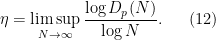
We will call this the upper exponent of 


for any sufficiently small

for any 

Applying (8) we then have

If we choose 


Exercise 8 Show that one still obtains a subpolynomial upper bound if the estimate (10) is replaced with
for some constant
, so long as we also improve (9) to
(This variant of the argument lets one handle the non-endpoint cases
of the decoupling theorem for the paraboloid.)

To establish decoupling estimates for the moment curve, restricting to the endpoint case 


- (Crude upper bound for
- (Multilinear reduction, using non-isotropic rescaling) For any
- (Crude upper bound for
- (Hölder) For
and
one has
and also
whenever, where
.
- (Rescaled decoupling hypothesis) For
- (Lower dimensional decoupling) If
and
, then
- (Multilinear Kakeya) If
, then


It is now substantially less obvious that these estimates can be combined to demonstrate that
These examples indicate a general strategy to establish that some quantity
- (i) Introducing some family of related auxiliary quantities, often parameterised by several further parameters;
- (ii) establishing as many bounds between these quantities and the original quantity
- (iii) appealing to some sort of “induction on scales” to conclude.
The first two steps (i), (ii) depend very much on the harmonic analysis nature of the quantities
In this post I would like to observe that one can clean up and made more systematic this final step (iii) by passing to upper exponents (12) to eliminate the role of the parameter
For instance, if

from which it is immediate that 
Exercise 9 Repeat Exercise 7 using this method.
Similarly, given the quantities 


for any 


For any natural number 


Now suppose that 


for all 
Assume for contradiction that 

At this point we can eliminate the role of

then on taking limit superiors of the previous inequalities we conclude that

for all 

so that 


This leads to a contradiction when
Exercise 10 Redo Exercise 8 using this method.
The same strategy now clarifies how to proceed with the more complicated system of quantities 


for all

for

for
As before, if we assume for sake of contradiction that

We can then again eliminate the role of 

and thus getting the simplified axiom system


and also

for

for
In view of the latter two estimates it is natural to restrict attention to the quantities 


The axioms now simplify to


 , and
, and 
for
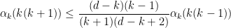
It turns out that the inequality (27) is strongest when 

for
From the last two inequalities (28), (29) we see that a special role is likely to be played by the exponents
for 
for 

for
Similarly, from (25) and a brief calculation we have

for 


for

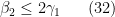
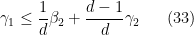
Let us write out the system of equations we have obtained in full:
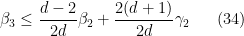


We can then eliminate the variables one by one. Inserting (33) into (32) we obtain
which simplifies to
Inserting this into (34) gives

which when combined with (35) gives
which simplifies to
Iterating this we get

for all
for all

which on insertion into (36), (37) gives

which is absurd if
Remark 11 (This observation is essentially due to Heath-Brown.) If we let
(arranged in whatever order one pleases), then the above system of inequalities (32)–(36) (using (37) to handle the appearance of
in (36)) reads
for some explicit square matrix
with non-negative coefficients, where the inequality denotes pointwise domination, and
is an explicit vector with non-positive coefficients that reflects the effect of (37). It is possible to show (using (24), (26)) that all the coefficients of
for any natural number
would now grow exponentially; this is typically the situation for “non-endpoint” applications such as proving decoupling inequalities away from the endpoint. In the endpoint situation discussed above, the Perron-Frobenius eigenvalue is
now grows at least linearly, which still gives the required contradiction for any
is the spectral radius of
is a left Perron-Frobenius eigenvector, that is to say a non-negative vector, not identically zero, such that
, then by taking inner products of (38) with
we obtain
If
this leads to a contradiction since
is negative and
is non-positive. When
one still gets a contradiction as long as

Remark 12 (This calculation is essentially due to Guo and Zorin-Kranich.) Here is a concrete application of the Perron-Frobenius strategy outlined above to the system of inequalities (32)–(37). Consider the weighted sum
I had secretly calculated the weights
,
as coming from the left Perron-Frobenius eigenvector of the matrix
is bounded by
(with the convention that the
term is absent); this simplifies after some calculation to the bound
and this and (37) then leads to the required contradiction.


Exercise 13
- (i) Extend the above analysis to also cover the non-endpoint case
. (One will need to establish the claim
for
.)
- (ii) Modify the argument to deal with the remaining cases
by dropping some of the steps.
[UPDATE, Feb 1, 2021: the strategy sketched out below has been successfully implemented to rigorously obtain the desired implication in this recent preprint of Giulio Bresciani.]
I recently came across this question on MathOverflow asking if there are any polynomials 
On the other hand, the one surviving response to the question does point out this paper of Poonen which shows that assuming a powerful conjecture in Diophantine geometry known as the Bombieri-Lang conjecture (discussed in this previous post), it is at least possible to exhibit polynomials
I believe that it should be possible to also rule out the existence of bijective polynomials
Here is how I imagine a Bombieri-Lang-powered resolution of this question should proceed (modulo a large number of unjustified and somewhat vague steps that I believe to be true but have not established rigorously). Suppose for contradiction that we have a bijective polynomial 

has infinitely many rational points; indeed, every rational 

- (a) The rational points in
- (b) The rational points in
Consider case (b) first. By definition, this case asserts that the rational points in 

- (i) If
is birational to an elliptic curve, then the number of elements of
of height at most
should grow at most polylogarithmically in
.
- (ii) If
for some rational
, then then the number of elements of
(in fact I think it can only grow like
).
I do not have proofs of these results (though I think something similar to (i) can be found in Knapp’s book, and (ii) should basically follow by using a rational parameterisation 


for all 


for some rational functions 


This leaves the scenario in which case (a) holds for a “positive fraction” of 


Recent Comments