Sums of GUE matrices and concentration of hives from correlation decay of eigengaps

Hariharan Narayanan, Scott Sheffield, and I have just uploaded to the arXiv our paper “Sums of GUE matrices and concentration of hives from correlation decay of eigengaps“. This is a personally satisfying paper for me, as it connects the work I did as a graduate student (with Allen Knutson and Chris Woodward) on sums of Hermitian matrices, with more recent work I did (with Van Vu) on random matrix theory, as well as several other results by other authors scattered across various mathematical subfields.

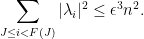
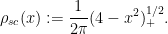
Suppose are two Hermitian matrices with eigenvalues and respectively (arranged in non-increasing order. What can one say about the eigenvalues of the sum ? There are now many ways to answer this question precisely; one of them, introduced by Allen and myself many years ago, is that there exists a certain triangular array of numbers called a “hive” that has as its boundary values. On the other hand, by the pioneering work of Voiculescu in free probability, we know in the large limit that if are asymptotically drawn from some limiting distribution, and and are drawn independently at random (using the unitarily invariant Haar measure) amongst all Hermitian matrices with the indicated eigenvalues, then (under mild hypotheses on the distribution, and under suitable normalization), will almost surely have a limiting distribution that is the free convolution of the two original distributions.

One of my favourite open problems is to come up with a theory of “free hives” that allows one to explain the latter fact from the former. This is still unresolved, but we are now beginning to make a bit of progress towards this goal. We know (for instance from the calculations of Coquereaux and Zuber) that if are drawn independently at random with eigenvalues , then the eigenvalues of are distributed according to the boundary values of an “augmented hive” with two boundaries , drawn uniformly at random from the polytope of all such augmented hives. (This augmented hive is basically a regular hive with another type of pattern, namely a Gelfand-Tsetlin pattern, glued to one side of it.) So, if one could show some sort of concentration of measure for the entries of this augmented hive, and calculate what these entries concentrated to, one should presumably be able to recover Voiculescu’s result after some calculation.

In this paper, we are able to accomplish the first half of this goal, assuming that the spectra are not deterministic, but rather drawn from the spectra of rescaled GUE matrices (thus are independent rescaled copies of the GUE ensemble). We have chosen to normalize matters so that the eigenvalues have size , so that the entries of the augmented hive have entries . Our result is then that the entries of the augmented hive in fact have a standard deviation of , thus exhibiting a little bit of concentration. (Actually, from the Brunn-Minkowski inequality, the distribution of these entries is log concave, so once once controls the standard deviation one also gets a bit of exponential decay beyond the standard deviation; Narayanan and Sheffield had also recently established the existence of a rate function for this sort of model.) Presumably one should get much better concentration, and one should be able to handle other models than the GUE ensemble, but this is the first advance that we were able to achieve.

Augmented hives seem tricky to work with directly, but by adapting the octahedron recurrence introduced for this problem by Knutson, Woodward, and myself some time ago (which is related to the associativity of addition for Hermitian matrices), one can construct a piecewise linear volume-preserving map between the cone of augmented hives, and the product of two Gelfand-Tsetlin cones. The problem then reduces to establishing concentration of measure for certain piecewise linear maps on products of Gelfand-Tsetlin cones (endowed with a certain GUE-type measure). This is a promising formulation because Gelfand-Tsetlin cones are by now quite well understood.

On the other hand, the piecewise linear map, initially defined by iterating the octahedron relation , looks somewhat daunting. Fortunately, there is an explicit formulation of this map due to Speyer, as the supremum of certain linear maps associated to perfect matchings of a certain “excavation graph”. For us it was convenient to work with the dual of this excavation graph, and associate these linear maps to certain “lozenge tilings” of a hexagon.

It would be more convenient to study the concentration of each linear map separately, rather than their supremum. By the Cheeger inequality, it turns out that one can relate the latter to the former provided that one has good control on the Cheeger constant of the underlying measure on the Gelfand-Tsetlin cones. Fortunately, the measure is log-concave, so one can use the very recent work of Klartag on the KLS conjecture to eliminate the supremum (up to a logarithmic loss which is only moderately annoying to deal with).

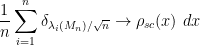
It remains to obtain concentration on the linear map associated to a given lozenge tiling. After stripping away some contributions coming from lozenges near the edge (using some eigenvalue rigidity results of Van Vu and myself), one is left with some bulk contributions which ultimately involve eigenvalue interlacing gaps such as

where is the eigenvalue of the top left minor of , and is in the bulk region for some fixed . To get the desired result, one needs some non-trivial correlation decay in for these statistics. If one was working with eigenvalue gaps rather than interlacing results, then such correlation decay was conveniently obtained for us by recent work of Cippoloni, Erdös, and Schröder. So the last remaining challenge is to understand the relation between eigenvalue gaps and interlacing gaps.

For this we turned to the work of Metcalfe, who uncovered a determinantal process structure to this problem, with a kernel associated to Lagrange interpolation polynomials. It is possible to satisfactorily estimate various integrals of these kernels using the residue theorem and eigenvalue rigidity estimates, thus completing the required analysis.

Eigenvectors from Eigenvalues: a survey of a basic identity in linear algebra

Peter Denton, Stephen Parke, Xining Zhang, and I have just uploaded to the arXiv a completely rewritten version of our previous paper, now titled “Eigenvectors from Eigenvalues: a survey of a basic identity in linear algebra“. This paper is now a survey of the various literature surrounding the following basic identity in linear algebra, which we propose to call the eigenvector-eigenvalue identity:

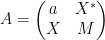
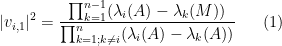
Theorem 1 (Eigenvector-eigenvalue identity) Let be an Hermitian matrix, with eigenvalues . Let be a unit eigenvector corresponding to the eigenvalue , and let be the component of . Then

where is the Hermitian matrix formed by deleting the row and column from .

When we posted the first version of this paper, we were unaware of previous appearances of this identity in the literature; a related identity had been used by Erdos-Schlein-Yau and by myself and Van Vu for applications to random matrix theory, but to our knowledge this specific identity appeared to be new. Even two months after our preprint first appeared on the arXiv in August, we had only learned of one other place in the literature where the identity showed up (by Forrester and Zhang, who also cite an earlier paper of Baryshnikov).

The situation changed rather dramatically with the publication of a popular science article in Quanta on this identity in November, which gave this result significantly more exposure. Within a few weeks we became informed (through private communication, online discussion, and exploration of the citation tree around the references we were alerted to) of over three dozen places where the identity, or some other closely related identity, had previously appeared in the literature, in such areas as numerical linear algebra, various aspects of graph theory (graph reconstruction, chemical graph theory, and walks on graphs), inverse eigenvalue problems, random matrix theory, and neutrino physics. As a consequence, we have decided to completely rewrite our article in order to collate this crowdsourced information, and survey the history of this identity, all the known proofs (we collect seven distinct ways to prove the identity (or generalisations thereof)), and all the applications of it that we are currently aware of. The citation graph of the literature that this ad hoc crowdsourcing effort produced is only very weakly connected, which we found surprising:

The earliest explicit appearance of the eigenvector-eigenvalue identity we are now aware of is in a 1966 paper of Thompson, although this paper is only cited (directly or indirectly) by a fraction of the known literature, and also there is a precursor identity of Löwner from 1934 that can be shown to imply the identity as a limiting case. At the end of the paper we speculate on some possible reasons why this identity only achieved a modest amount of recognition and dissemination prior to the November 2019 Quanta article.

Eigenvectors from eigenvalues

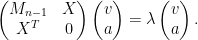
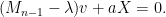
Peter Denton, Stephen Parke, Xining Zhang, and I have just uploaded to the arXiv the short unpublished note “Eigenvectors from eigenvalues“. This note gives two proofs of a general eigenvector identity observed recently by Denton, Parke and Zhang in the course of some quantum mechanical calculations. The identity is as follows:

Theorem 1 Let be an Hermitian matrix, with eigenvalues . Let be a unit eigenvector corresponding to the eigenvalue , and let be the component of . Then

where is the Hermitian matrix formed by deleting the row and column from .

For instance, if we have

for some real number , -dimensional vector , and Hermitian matrix , then we have

assuming that the denominator is non-zero.

Once one is aware of the identity, it is not so difficult to prove it; we give two proofs, each about half a page long, one of which is based on a variant of the Cauchy-Binet formula, and the other based on properties of the adjugate matrix. But perhaps it is surprising that such a formula exists at all; one does not normally expect to learn much information about eigenvectors purely from knowledge of eigenvalues. In the random matrix theory literature, for instance in this paper of Erdos, Schlein, and Yau, or this later paper of Van Vu and myself, a related identity has been used, namely

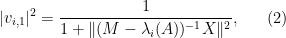
but it is not immediately obvious that one can derive the former identity from the latter. (I do so below the fold; we ended up not putting this proof in the note as it was longer than the two other proofs we found. I also give two other proofs below the fold, one from a more geometric perspective and one proceeding via Cramer’s rule.) It was certainly something of a surprise to me that there is no explicit appearance of the components of in the formula (1) (though they do indirectly appear through their effect on the eigenvalues ; for instance from taking traces one sees that ).

One can get some feeling of the identity (1) by considering some special cases. Suppose for instance that is a diagonal matrix with all distinct entries. The upper left entry of is one of the eigenvalues of . If it is equal to , then the eigenvalues of are the other eigenvalues of , and now the left and right-hand sides of (1) are equal to . At the other extreme, if is equal to a different eigenvalue of , then now appears as an eigenvalue of , and both sides of (1) now vanish. More generally, if we order the eigenvalues and , then the Cauchy interlacing inequalities tell us that

for , and

for , so that the right-hand side of (1) lies between and , which is of course consistent with (1) as is a unit vector. Thus the identity relates the coefficient sizes of an eigenvector with the extent to which the Cauchy interlacing inequalities are sharp.

Random matrices: tail bounds for gaps between eigenvalues

Hoi Nguyen, Van Vu, and myself have just uploaded to the arXiv our paper “Random matrices: tail bounds for gaps between eigenvalues“. This is a followup paper to my recent paper with Van in which we showed that random matrices of Wigner type (such as the adjacency matrix of an Erdös-Renyi graph) asymptotically almost surely had simple spectrum. In the current paper, we push the method further to show that the eigenvalues are not only distinct, but are (with high probability) separated from each other by some negative power of . This follows the now standard technique of replacing any appearance of discrete Littlewood-Offord theory (a key ingredient in our previous paper) with its continuous analogue (inverse theorems for small ball probability). For general Wigner-type matrices (in which the matrix entries are not normalised to have mean zero), we can use the inverse Littlewood-Offord theorem of Nguyen and Vu to obtain (under mild conditions on ) a result of the form

for any and , if is sufficiently large depending on (in a linear fashion), and is sufficiently large depending on . The point here is that can be made arbitrarily large, and also that no continuity or smoothness hypothesis is made on the distribution of the entries. (In the continuous case, one can use the machinery of Wegner estimates to obtain results of this type, as was done in a paper of Erdös, Schlein, and Yau.)

In the mean zero case, it becomes more efficient to use an inverse Littlewood-Offord theorem of Rudelson and Vershynin to obtain (with the normalisation that the entries of have unit variance, so that the eigenvalues of are with high probability), giving the bound

for (one also has good results of this type for smaller values of ). This is only optimal in the regime ; we expect to establish some eigenvalue repulsion, improving the RHS to for real matrices and for complex matrices, but this appears to be a more difficult task (possibly requiring some quadratic inverse Littlewood-Offord theory, rather than just linear inverse Littlewood-Offord theory). However, we can get some repulsion if one works with larger gaps, getting a result roughly of the form

for any fixed and some absolute constant (which we can asymptotically make to be for large , though it ought to be as large as ), by using a higher-dimensional version of the Rudelson-Vershynin inverse Littlewood-Offord theorem.

In the case of Erdös-Renyi graphs, we don’t have mean zero and the Rudelson-Vershynin Littlewood-Offord theorem isn’t quite applicable, but by working carefully through the approach based on the Nguyen-Vu theorem we can almost recover (1), except for a loss of on the RHS.

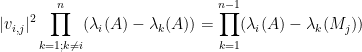
As a sample applications of the eigenvalue separation results, we can now obtain some information about eigenvectors; for instance, we can show that the components of the eigenvectors all have magnitude at least for some with high probability. (Eigenvectors become much more stable, and able to be studied in isolation, once their associated eigenvalue is well separated from the other eigenvalues; see this previous blog post for more discussion.)

Random matrices have simple spectrum

Van Vu and I have just uploaded to the arXiv our paper “Random matrices have simple spectrum“. Recall that an Hermitian matrix is said to have simple eigenvalues if all of its eigenvalues are distinct. This is a very typical property of matrices to have: for instance, as discussed in this previous post, in the space of all Hermitian matrices, the space of matrices without all eigenvalues simple has codimension three, and for real symmetric cases this space has codimension two. In particular, given any random matrix ensemble of Hermitian or real symmetric matrices with an absolutely continuous distribution, we conclude that random matrices drawn from this ensemble will almost surely have simple eigenvalues.

For discrete random matrix ensembles, though, the above argument breaks down, even though general universality heuristics predict that the statistics of discrete ensembles should behave similarly to those of continuous ensembles. A model case here is the adjacency matrix of an Erdös-Rényi graph – a graph on vertices in which any pair of vertices has an independent probability of being in the graph. For the purposes of this paper one should view as fixed, e.g. , while is an asymptotic parameter going to infinity. In this context, our main result is the following (answering a question of Babai):

Theorem 1 With probability , has simple eigenvalues.

Our argument works for more general Wigner-type matrix ensembles, but for sake of illustration we will stick with the Erdös-Renyi case. Previous work on local universality for such matrix models (e.g. the work of Erdos, Knowles, Yau, and Yin) was able to show that any individual eigenvalue gap did not vanish with probability (in fact for some absolute constant ), but because there are different gaps that one has to simultaneously ensure to be non-zero, this did not give Theorem 1 as one is forced to apply the union bound.

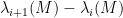
Our argument in fact gives simplicity of the spectrum with probability for any fixed ; in a subsequent paper we also show that it gives a quantitative lower bound on the eigenvalue gaps (analogous to how many results on the singularity probability of random matrices can be upgraded to a bound on the least singular value).

The basic idea of argument can be sketched as follows. Suppose that has a repeated eigenvalue . We split

for a random minor and a random sign vector ; crucially, and are independent. If has a repeated eigenvalue , then by the Cauchy interlacing law, also has an eigenvalue . We now write down the eigenvector equation for at :

Extracting the top coefficients, we obtain

If we let be the -eigenvector of , then by taking inner products with we conclude that

we typically expect to be non-zero, in which case we arrive at

In other words, in order for to have a repeated eigenvalue, the top right column of has to be orthogonal to an eigenvector of the minor . Note that and are going to be independent (once we specify which eigenvector of to take as ). On the other hand, thanks to inverse Littlewood-Offord theory (specifically, we use an inverse Littlewood-Offord theorem of Nguyen and Vu), we know that the vector is unlikely to be orthogonal to any given vector independent of , unless the coefficients of are extremely special (specifically, that most of them lie in a generalised arithmetic progression). The main remaining difficulty is then to show that eigenvectors of a random matrix are typically not of this special form, and this relies on a conditioning argument originally used by Komlós to bound the singularity probability of a random sign matrix. (Basically, if an eigenvector has this special form, then one can use a fraction of the rows and columns of the random matrix to determine the eigenvector completely, while still preserving enough randomness in the remaining portion of the matrix so that this vector will in fact not be an eigenvector with high probability.)

The spectral proof of the Szemeredi regularity lemma

Perhaps the most important structural result about general large dense graphs is the Szemerédi regularity lemma. Here is a standard formulation of that lemma:

Lemma 1 (Szemerédi regularity lemma) Let be a graph on vertices, and let . Then there exists a partition for some with the property that for all but at most of the pairs , the pair is -regular in the sense that

whenever are such that and , and is the edge density between and . Furthermore, the partition is equitable in the sense that for all .

There are many proofs of this lemma, which is actually not that difficult to establish; see for instance these previous blog posts for some examples. In this post I would like to record one further proof, based on the spectral decomposition of the adjacency matrix of , which is essentially due to Frieze and Kannan. (Strictly speaking, Frieze and Kannan used a variant of this argument to establish a weaker form of the regularity lemma, but it is not difficult to modify the Frieze-Kannan argument to obtain the usual form of the regularity lemma instead. Some closely related spectral regularity lemmas were also developed by Szegedy.) I found recently (while speaking at the Abel conference in honour of this year’s laureate, Endre Szemerédi) that this particular argument is not as widely known among graph theory experts as I had thought, so I thought I would record it here.

For reasons of exposition, it is convenient to first establish a slightly weaker form of the lemma, in which one drops the hypothesis of equitability (but then has to weight the cells by their magnitude when counting bad pairs):

Lemma 2 (Szemerédi regularity lemma, weakened variant) . Let be a graph on vertices, and let . Then there exists a partition for some with the property that for all pairs outside of an exceptional set , one has

whenever , for some real number , where is the number of edges between and . Furthermore, we have

Let us now prove Lemma 2. We enumerate (after relabeling) as . The adjacency matrix of the graph is then a self-adjoint matrix, and thus admits an eigenvalue decomposition

for some orthonormal basis of and some eigenvalues , which we arrange in decreasing order of magnitude:

We can compute the trace of as

But we also have , so

Among other things, this implies that

for all .

Let be a function (depending on ) to be chosen later, with for all . Applying (3) and the pigeonhole principle (or the finite convergence principle, see this blog post), we can find such that

(Indeed, the bound on is basically iterated times.) We can now split

where is the “structured” component

is the “small” component

and is the “pseudorandom” component

We now design a vertex partition to make approximately constant on most cells. For each , we partition into cells on which (viewed as a function from to ) only fluctuates by , plus an exceptional cell of size coming from the values where is excessively large (larger than ). Combining all these partitions together, we can write for some , where has cardinality at most , and for all , the eigenfunctions all fluctuate by at most . In particular, if , then (by (4) and (6)) the entries of fluctuate by at most on each block . If we let be the mean value of these entries on , we thus have

for any and , where we view the indicator functions as column vectors of dimension .

Next, we observe from (3) and (7) that . If we let be the coefficients of , we thus have

and hence by Markov’s inequality we have

for all pairs outside of an exceptional set with

If avoids , we thus have

for any , by (10) and the Cauchy-Schwarz inequality.

Finally, to control we see from (4) and (8) that has an operator norm of at most . In particular, we have from the Cauchy-Schwarz inequality that

for any .

Let be the set of all pairs where either , , , or

One easily verifies that (2) holds. If is not in , then by summing (9), (11), (12) and using (5), we see that

for all . The left-hand side is just . As , we have

and so (since )

If we let be a sufficiently rapidly growing function of that depends on , the second error term in (13) can be absorbed in the first, and (1) follows. This concludes the proof of Lemma 2.

To prove Lemma 1, one argues similarly (after modifying as necessary), except that the initial partition of constructed above needs to be subdivided further into equitable components (of size ), plus some remainder sets which can be aggregated into an exceptional component of size (and which can then be redistributed amongst the other components to arrive at a truly equitable partition). We omit the details.

Remark 1 It is easy to verify that needs to be growing exponentially in in order for the above argument to work, which leads to tower-exponential bounds in the number of cells in the partition. It was shown by Gowers that a tower-exponential bound is actually necessary here. By varying , one basically obtains the strong regularity lemma first established by Alon, Fischer, Krivelevich, and Szegedy; in the opposite direction, setting essentially gives the weak regularity lemma of Frieze and Kannan.

Remark 2 If we specialise to a Cayley graph, in which is a finite abelian group and for some (symmetric) subset of , then the eigenvectors are characters, and one essentially recovers the arithmetic regularity lemma of Green, in which the vertex partition classes are given by Bohr sets (and one can then place additional regularity properties on these Bohr sets with some additional arguments). The components of , representing high, medium, and low eigenvalues of , then become a decomposition associated to high, medium, and low Fourier coefficients of .

Remark 3 The use of spectral theory here is parallel to the use of Fourier analysis to establish results such as Roth’s theorem on arithmetic progressions of length three. In analogy with this, one could view hypergraph regularity as being a sort of “higher order spectral theory”, although this spectral perspective is not as convenient as it is in the graph case.

Random matrices: Sharp concentration of eigenvalues

Van Vu and I have just uploaded to the arXiv our paper Random matrices: Sharp concentration of eigenvalues, submitted to the Electronic Journal of Probability. As with many of our previous papers, this paper is concerned with the distribution of the eigenvalues of a random Wigner matrix (such as a matrix drawn from the Gaussian Unitary Ensemble (GUE) or Gaussian Orthogonal Ensemble (GOE)). To simplify the discussion we shall mostly restrict attention to the bulk of the spectrum, i.e. to eigenvalues with for some fixed , although analogues of most of the results below have also been obtained at the edge of the spectrum.

If we normalise the entries of the matrix to have mean zero and variance , then in the asymptotic limit , we have the Wigner semicircle law, which asserts that the eigenvalues are asymptotically distributed according to the semicircular distribution , where

An essentially equivalent way of saying this is that for large , we expect the eigenvalue of to stay close to the classical location , defined by the formula

In particular, from the Wigner semicircle law it can be shown that asymptotically almost surely, one has

for all .

In the modern study of the spectrum of Wigner matrices (and in particular as a key tool in establishing universality results), it has become of interest to improve the error term in (1) as much as possible. A typical early result in this direction was by Bai, who used the Stieltjes transform method to obtain polynomial convergence rates of the shape for some absolute constant ; see also the subsequent papers of Alon-Krivelevich-Vu and of of Meckes, who were able to obtain such convergence rates (with exponentially high probability) by using concentration of measure tools, such as Talagrand’s inequality. On the other hand, in the case of the GUE ensemble it is known (by this paper of Gustavsson) that has variance comparable to in the bulk, so that the optimal error term in (1) should be about . (One may think that if one wanted bounds on (1) that were uniform in , one would need to enlarge the error term further, but this does not appear to be the case, due to strong correlations between the ; note for instance this recent result of Ben Arous and Bourgarde that the largest gap between eigenvalues in the bulk is typically of order .)

A significant advance in this direction was achieved by Erdos, Schlein, and Yau in a series of papers where they used a combination of Stieltjes transform and concentration of measure methods to obtain local semicircle laws which showed, among other things, that one had asymptotics of the form

with exponentially high probability for intervals in the bulk that were as short as for some , where is the number of eigenvalues. These asymptotics are consistent with a good error term in (1), and are already sufficient for many applications, but do not quite imply a strong concentration result for individual eigenvalues (basically because they do not preclude long-range or “secular” shifts in the spectrum that involve large blocks of eigenvalues at mesoscopic scales). Nevertheless, this was rectified in a subsequent paper of Erdos, Yau, and Yin, which roughly speaking obtained a bound of the form

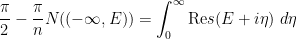
in the bulk with exponentially high probability, for Wigner matrices obeying some exponential decay conditions on the entries. This was achieved by a rather delicate high moment calculation, in which the contribution of the diagonal entries of the resolvent (whose average forms the Stieltjes transform) was shown to mostly cancel each other out.

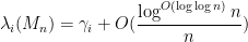
As the GUE computations show, this concentration result is sharp up to the quasilogarithmic factor . The main result of this paper is to improve the concentration result to one more in line with the GUE case, namely

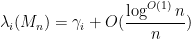
with exponentially high probability (see the paper for a more precise statement of results). The one catch is that an additional hypothesis is required, namely that the entries of the Wigner matrix have vanishing third moment. We also obtain similar results for the edge of the spectrum (but with a different scaling).

Our arguments are rather different from those of Erdos, Yau, and Yin, and thus provide an alternate approach to establishing eigenvalue concentration. The main tool is the Lindeberg exchange strategy, which is also used to prove the Four Moment Theorem (although we do not directly invoke the Four Moment Theorem in our analysis). The main novelty is that this exchange strategy is now used to establish large deviation estimates (i.e. exponentially small tail probabilities) rather than universality of the limiting distribution. Roughly speaking, the basic point is as follows. The Lindeberg exchange strategy seeks to compare a function of many independent random variables with the same function of a different set of random variables (which match moments with the original set of variables to some order, such as to second or fourth order) by exchanging the random variables one at a time. Typically, one tries to upper bound expressions such as

for various smooth test functions , by performing a Taylor expansion in the variable being swapped and taking advantage of the matching moment hypotheses. In previous implementations of this strategy, was a bounded test function, which allowed one to get control of the bulk of the distribution of , and in particular in controlling probabilities such as

for various thresholds and , but did not give good control on the tail as the error terms tended to be polynomially decaying in rather than exponentially decaying. However, it turns out that one can modify the exchange strategy to deal with moments such as

for various moderately large (e.g. of size comparable to ), obtaining results such as

after performing all the relevant exchanges. As such, one can then use large deviation estimates on to deduce large deviation estimates on .

In this paper we also take advantage of a simplification, first noted by Erdos, Yau, and Yin, that Four Moment Theorems become somewhat easier to prove if one works with resolvents (and the closely related Stieltjes transform ) rather than with individual eigenvalues, as the Taylor expansion of resolvents are very simple (essentially being a Neumann series). The relationship between the Stieltjes transform and the location of individual eigenvalues can be seen by taking advantage of the identity

for any energy level , which can be verified from elementary calculus. (In practice, we would truncate near zero and near infinity to avoid some divergences, but this is a minor technicality.) As such, a concentration result for the Stieltjes transform can be used to establish an analogous concentration result for the eigenvalue counting functions , which in turn can be used to deduce concentration results for individual eigenvalues by some basic combinatorial manipulations.

Random matrices: Localization of the eigenvalues and the necessity of four moments

Van Vu and I have just uploaded to the arXiv our paper “Random matrices: Localization of the eigenvalues and the necessity of four moments“, submitted to Probability Theory and Related Fields. This paper concerns the distribution of the eigenvalues

of a Wigner random matrix . More specifically, we consider Hermitian random matrices whose entries have mean zero and variance one, with the upper-triangular portion of the matrix independent, with the diagonal elements iid, and the real and imaginary parts of the strictly upper-triangular portion of the matrix iid. For technical reasons we also assume that the distribution of the coefficients decays exponentially or better. Examples of Wigner matrices include the Gaussian Unitary Ensemble (GUE) and random symmetric complex Bernoulli matrices (which equal on the diagonal, and off the diagonal). The Gaussian Orthogonal Ensemble (GOE) is also an example once one makes the minor change of setting the diagonal entries to have variance two instead of one.

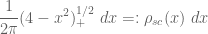
The most fundamental theorem about the distribution of these eigenvalues is the Wigner semi-circular law, which asserts that (almost surely) one has

(in the vague topology) where is the semicircular distribution. (See these lecture notes on this blog for more discusssion of this law.)

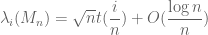
One can phrase this law in a number of equivalent ways. For instance, in the bulk region , one almost surely has

uniformly for in , where the classical location of the (normalised) eigenvalue is defined by the formula

The bound (1) also holds in the edge case (by using the operator norm bound , due to Bai and Yin), but for sake of exposition we shall restriction attention here only to the bulk case.

From (1) we see that the semicircular law controls the eigenvalues at the coarse scale of . There has been a significant amount of work in the literature in obtaining control at finer scales, and in particular at the scale of the average eigenvalue spacing, which is of the order of . For instance, we now have a universal limit theorem for the normalised eigenvalue spacing in the bulk for all Wigner matrices, a result of Erdos, Ramirez, Schlein, Vu, Yau, and myself. One tool for this is the four moment theorem of Van and myself, which roughly speaking shows that the behaviour of the eigenvalues at the scale (and even at the slightly finer scale of for some absolute constant ) depends only on the first four moments of the matrix entries. There is also a slight variant, the three moment theorem, which asserts that the behaviour of the eigenvalues at the slightly coarser scale of depends only on the first three moments of the matrix entries.

It is natural to ask whether these moment conditions are necessary. From the result of Erdos, Ramirez, Schlein, Vu, Yau, and myself, it is known that to control the eigenvalue spacing at the critical scale , no knowledge of any moments beyond the second (i.e. beyond the mean and variance) are needed. So it is natural to conjecture that the same is true for the eigenvalues themselves.

The main result of this paper is to show that this is not the case; that at the critical scale , the distribution of eigenvalues is sensitive to the fourth moment, and so the hypothesis of the four moment theorem cannot be relaxed.

Heuristically, the reason for this is easy to explain. One begins with an inspection of the expected fourth moment

A standard moment method computation shows that the right hand side is equal to

where is the fourth moment of the real part of the off-diagonal coefficients of . In particular, a change in the fourth moment by leads to a change in the expression by . Thus, for a typical , one expects to shift by ; since on the average, we thus expect itself to shift by about by the mean-value theorem.

To make this rigorous, one needs a sufficiently strong concentration of measure result for that keeps it close to its mean value. There are already a number of such results in the literature. For instance, Guionnet and Zeitouni showed that was sharply concentrated around an interval of size around for any (in the sense that the probability that one was outside this interval was exponentially small). In one of my papers with Van, we showed that was also weakly concentrated around an interval of size around , in the sense that the probability that one was outside this interval was for some absolute constant . Finally, if one made an additional log-Sobolev hypothesis on the entries, it was shown by by Erdos, Yau, and Yin that the average variance of as varied from to was of the size of for some absolute .

As it turns out, the first two concentration results are not sufficient to justify the previous heuristic argument. The Erdos-Yau-Yin argument suffices, but requires a log-Sobolev hypothesis. In our paper, we argue differently, using the three moment theorem (together with the theory of the eigenvalues of GUE, which is extremely well developed) to show that the variance of each individual is (without averaging in ). No log-Sobolev hypothesis is required, but instead we need to assume that the third moment of the coefficients vanishes (because we want to use the three moment theorem to compare the Wigner matrix to GUE, and the coefficients of the latter have a vanishing third moment). From this we are able to make the previous arguments rigorous, and show that the mean is indeed sensitive to the fourth moment of the entries at the critical scale .

One curious feature of the analysis is how differently the median and the mean of the eigenvalue react to the available technology. To control the global behaviour of the eigenvalues (after averaging in ), it is much more convenient to use the mean, and we have very precise control on global averages of these means thanks to the moment method. But to control local behaviour, it is the median which is much better controlled. For instance, we can localise the median of to an interval of size , but can only localise the mean to a much larger interval of size . Ultimately, this is because with our current technology there is a possible exceptional event of probability as large as for which all eigenvalues could deviate as far as from their expected location, instead of their typical deviation of . The reason for this is technical, coming from the fact that the four moment theorem method breaks down when two eigenvalues are very close together (less than times the average eigenvalue spacing), and so one has to cut out this event, which occurs with a probability of the shape . It may be possible to improve the four moment theorem proof to be less sensitive to eigenvalue near-collisions, in which case the above bounds are likely to improve.

Random matrices: universality of local eigenvalue statistics

Van Vu and I have just uploaded to the arXiv our paper “Random matrices: universality of local eigenvalue statistics“, submitted to Acta Math..  This paper concerns the eigenvalues of a Wigner matrix , which we define to be a random Hermitian matrix whose upper-triangular entries are independent (and whose strictly upper-triangular entries are also identically distributed).  [The lower-triangular entries are of course determined from the upper-triangular ones by the Hermitian property.]  We normalise the matrices so that all the entries have mean zero and variance 1.  Basic examples of Wigner Hermitian matrices include

1. The Gaussian Unitary Ensemble (GUE), in which the upper-triangular entries are complex gaussian, and the diagonal entries are real gaussians;
2. The Gaussian Orthogonal Ensemble (GOE), in which all entries are real gaussian;
3. The Bernoulli Ensemble, in which all entries take values (with equal probability of each).

We will make a further distinction into Wigner real symmetric matrices (which are Wigner matrices with real coefficients, such as GOE and the Bernoulli ensemble) and Wigner Hermitian matrices (which are Wigner matrices whose upper-triangular coefficients have real and imaginary parts iid, such as GUE).

The GUE and GOE ensembles have a rich algebraic structure (for instance, the GUE distribution is invariant under conjugation by unitary matrices, while the GOE distribution is similarly invariant under conjugation by orthogonal matrices, hence the terminology), and as a consequence their eigenvalue distribution can be computed explicitly.  For instance, the joint distribution of the eigenvalues for GUE is given by the explicit formula

(0)

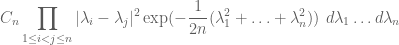
for some explicitly computable constant on the orthant (a result first established by Ginibre).  (A similar formula exists for GOE, but for simplicity we will just discuss GUE here.)  Using this explicit formula one can compute a wide variety of asymptotic eigenvalue statistics.  For instance, the (bulk) empirical spectral distribution (ESD) measure for GUE (and indeed for all Wigner matrices, see below) is known to converge (in the vague sense) to the Wigner semicircular law

(1)

as .  Actually, more precise statements are known for GUE; for instance, for , the eigenvalue is known to equal

(2)

with probability , where is the inverse cumulative distribution function of the semicircular law, thus

.

Furthermore, the distribution of the normalised eigenvalue spacing is known; in the bulk region for fixed , it converges as to the Gaudin distribution, which can be described explicitly in terms of determinants of the Dyson sine kernel .  Many further local statistics of the eigenvalues of GUE are in fact governed by this sine kernel, a result usually proven using the asymptotics of orthogonal polynomials (and specifically, the Hermite polynomials).  (At the edge of the spectrum, say , the asymptotic distribution is a bit different, being governed instead by the  Tracy-Widom law.)

It has been widely believed that these GUE facts enjoy a universality property, in the sense that they should also hold for wide classes of other matrix models. In particular, Wigner matrices should enjoy the same bulk distribution (1), the same asymptotic law (2) for individual eigenvalues, and the same sine kernel statistics as GUE. (The statistics for Wigner symmetric matrices are slightly different, and should obey GOE statistics rather than GUE ones.)

There has been a fair body of evidence to support this belief.  The bulk distribution (1) is in fact valid for all Wigner matrices (a result of Pastur, building on the original work of Wigner of course).  The Tracy-Widom statistics on the edge were established for all Wigner Hermitian matrices (assuming that the coefficients had a distribution which was symmetric and decayed exponentially) by Soshnikov (with some further refinements by Soshnikov and Peche).  Soshnikov’s arguments were based on an advanced version of the moment method.

The sine kernel statistics were established by Johansson for Wigner Hermitian matrices which were gaussian divisible, which means that they could be expressed as a non-trivial linear combination of another Wigner Hermitian matrix and an independent GUE.  (Basically, this means that distribution of the coefficients is a convolution of some other distribution with a gaussian.  There were some additional technical decay conditions in Johansson’s work which were removed in subsequent work of Ben Arous and Peche.)   Johansson’s work was based on an explicit formula for the joint distribution for gauss divisible matrices that generalises (0) (but is significantly more complicated).

Just last week, Erdos, Ramirez, Schlein, and Yau established sine kernel statistics for Wigner Hermitian matrices with exponential decay and a high degree of smoothness (roughly speaking, they require  control of up to six derivatives of the Radon-Nikodym derivative of the distribution).  Their method is based on an analysis of the dynamics of the eigenvalues under a smooth transition from a general Wigner Hermitian matrix to GUE, essentially a matrix version of the Ornstein-Uhlenbeck process, whose eigenvalue dynamics are governed by Dyson Brownian motion.

In my paper with Van, we establish similar results to that of Erdos et al. under slightly different hypotheses, and by a somewhat different method.  Informally, our main result is as follows:

Theorem 1. (Informal version)  Suppose is a Wigner Hermitian matrix whose coefficients have an exponentially decaying distribution, and whose real and imaginary parts are supported on at least three points (basically, this excludes Bernoulli-type distributions only) and have vanishing third moment (which is for instance the case for symmetric distributions).  Then one has the local statistics (2) (but with an error term of for any rather than ) and the sine kernel statistics for individual eigenvalue spacings (as well as higher order correlations) in the bulk.

If one removes the vanishing third moment hypothesis, one still has the sine kernel statistics provided one averages over all i.

There are analogous results for Wigner real symmetric matrices (see paper for details).  There are also some related results, such as a universal distribution for the least singular value of matrices of the form in Theorem 1, and a crude asymptotic for the determinant (in particular, with probability ).

The arguments are based primarily on the Lindeberg replacement strategy, which Van and I also used to obtain universality for the circular law for iid matrices, and for the least singular value for iid matrices, but also rely on other tools, such as some recent arguments of Erdos, Schlein, and Yau, as well as a very useful concentration inequality of Talagrand which lets us tackle both discrete and continuous matrix ensembles in a unified manner.  (I plan to talk about Talagrand’s inequality in my next blog post.)

When are eigenvalues stable?

I was asked recently (in relation to my recent work with Van Vu on the spectral theory of random matrices) to explain some standard heuristics regarding how the eigenvalues of an matrix A behave under small perturbations.  These heuristics can be summarised as follows:

1. For normal matrices (and in particular, unitary or self-adjoint matrices), eigenvalues are very stable under small perturbations.  For more general matrices, eigenvalues can become unstable if there is pseudospectrum present.
2. For self-adjoint (Hermitian) matrices, eigenvalues that are too close together tend to repel quickly from each other under such perturbations.  For more general matrices, eigenvalues can either be repelled or be attracted to each other, depending on the type of perturbation.

In this post I would like to briefly explain why these heuristics are plausible.