Polymath8b, II: Optimising the variational problem and the sieve

This is the second thread for the Polymath8b project to obtain new bounds for the quantity

either for small values of (in particular ) or asymptotically as . The previous thread may be found here. The currently best known bounds on are:

• (Maynard) .
• (Polymath8b, tentative) .
• (Polymath8b, tentative) for sufficiently large .
• (Maynard) Assuming the Elliott-Halberstam conjecture, , , and .

Following the strategy of Maynard, the bounds on proceed by combining four ingredients:

1. Distribution estimates or for the primes (or related objects);
2. Bounds for the minimal diameter of an admissible -tuple;
3. Lower bounds for the optimal value to a certain variational problem;
4. Sieve-theoretic arguments to convert the previous three ingredients into a bound on .

Accordingly, the most natural routes to improve the bounds on are to improve one or more of the above four ingredients.

Ingredient 1 was studied intensively in Polymath8a. The following results are known or conjectured (see the Polymath8a paper for notation and proofs):

• (Bombieri-Vinogradov) is true for all .
• (Polymath8a) is true for .
• (Polymath8a, tentative) is true for .
• (Elliott-Halberstam conjecture) is true for all .

Ingredient 2 was also studied intensively in Polymath8a, and is more or less a solved problem for the values of of interest (with exact values of for , and quite good upper bounds for for , available at this page). So the main focus currently is on improving Ingredients 3 and 4.

For Ingredient 3, the basic variational problem is to understand the quantity

for bounded measurable functions, not identically zero, on the simplex

with being the quadratic forms

and

Equivalently, one has

where is the positive semi-definite bounded self-adjoint operator

so is the operator norm of . Another interpretation of is that the probability that a rook moving randomly in the unit cube stays in simplex for moves is asymptotically .

We now have a fairly good asymptotic understanding of , with the bounds

holding for sufficiently large . There is however still room to tighten the bounds on for small ; I’ll summarise some of the ideas discussed so far below the fold.

For Ingredient 4, the basic tool is this:

Theorem 1 (Maynard) If is true and , then .

Thus, for instance, it is known that and , and this together with the Bombieri-Vinogradov inequality gives . This result is proven in Maynard’s paper and an alternate proof is also given in the previous blog post.

We have a number of ways to relax the hypotheses of this result, which we also summarise below the fold.

Polymath8b: Bounded intervals with many primes, after Maynard

For each natural number , let denote the quantity

where denotes the prime. In other words, is the least quantity such that there are infinitely many intervals of length that contain or more primes. Thus, for instance, the twin prime conjecture is equivalent to the assertion that , and the prime tuples conjecture would imply that is equal to the diameter of the narrowest admissible tuple of cardinality (thus we conjecturally have , , , , , and so forth; see this web page for further continuation of this sequence).

In 2004, Goldston, Pintz, and Yildirim established the bound conditional on the Elliott-Halberstam conjecture, which remains unproven. However, no unconditional finiteness of was obtained (although they famously obtained the non-trivial bound ), and even on the Elliot-Halberstam conjecture no finiteness result on the higher was obtained either (although they were able to show on this conjecture). In the recent breakthrough of Zhang, the unconditional bound was obtained, by establishing a weak partial version of the Elliott-Halberstam conjecture; by refining these methods, the Polymath8 project (which I suppose we could retroactively call the Polymath8a project) then lowered this bound to .

With the very recent preprint of James Maynard, we have the following further substantial improvements:

Theorem 1 (Maynard’s theorem) Unconditionally, we have the following bounds:

• .
• for an absolute constant and any .

If one assumes the Elliott-Halberstam conjecture, we have the following improved bounds:

• .
• .
• for an absolute constant and any .

The final conclusion on Elliott-Halberstam is not explicitly stated in Maynard’s paper, but follows easily from his methods, as I will describe below the fold. (At around the same time as Maynard’s work, I had also begun a similar set of calculations concerning , but was only able to obtain the slightly weaker bound unconditionally.) In the converse direction, the prime tuples conjecture implies that should be comparable to . Granville has also obtained the slightly weaker explicit bound for any by a slight modification of Maynard’s argument.

The arguments of Maynard avoid using the difficult partial results on (weakened forms of) the Elliott-Halberstam conjecture that were established by Zhang and then refined by Polymath8; instead, the main input is the classical Bombieri-Vinogradov theorem, combined with a sieve that is closer in spirit to an older sieve of Goldston and Yildirim, than to the sieve used later by Goldston, Pintz, and Yildirim on which almost all subsequent work is based.

The aim of the Polymath8b project is to obtain improved bounds on , and higher values of , either conditional on the Elliott-Halberstam conjecture or unconditional. The likeliest routes for doing this are by optimising Maynard’s arguments and/or combining them with some of the results from the Polymath8a project. This post is intended to be the first research thread for that purpose. To start the ball rolling, I am going to give below a presentation of Maynard’s results, with some minor technical differences (most significantly, I am using the Goldston-Pintz-Yildirim variant of the Selberg sieve, rather than the traditional “elementary Selberg sieve” that is used by Maynard (and also in the Polymath8 project), although it seems that the numerology obtained by both sieves is essentially the same). An alternate exposition of Maynard’s work has just been completed also by Andrew Granville.

Polymath8: Writing the first paper, V, and a look ahead

It’s time to (somewhat belatedly) roll over the previous thread on writing the first paper from the Polymath8 project, as this thread is overflowing with comments.  We are getting near the end of writing this large (173 pages!) paper, establishing a bound of 4,680 on the gap between primes, with only a few sections left to thoroughly proofread (and the last section should probably be removed, with appropriate changes elsewhere, in view of the more recent progress by Maynard).  As before, one can access the working copy of the paper at this subdirectory, as well as the rest of the directory, and the plan is to submit the paper to Algebra and Number theory (and the arXiv) once there is consensus to do so.  Even before this paper was submitted, it already has had some impact; Andrew Granville’s exposition of the bounded gaps between primes story for the Bulletin of the AMS follows several of the Polymath8 arguments in deriving the result.

After this paper is done, there is interest in continuing onwards with other Polymath8 – related topics, and perhaps it is time to start planning for them.  First of all, we have an invitation from  the Newsletter of the European Mathematical Society to discuss our experiences and impressions with the project.  I think it would be interesting to collect some impressions or thoughts (both positive and negative)  from people who were highly active in the research and/or writing aspects of the project, as well as from more casual participants who were following the progress more quietly.  This project seemed to attract a bit more attention than most other polymath projects (with the possible exception of the very first project, Polymath1).  I think there are several reasons for this; the project builds upon a recent breakthrough (Zhang’s paper) that attracted an impressive amount of attention and publicity; the objective is quite easy to describe, when compared against other mathematical research objectives; and one could summarise the current state of progress by a single natural number H, which implied by infinite descent that the project was guaranteed to terminate at some point, but also made it possible to set up a “scoreboard” that could be quickly and easily updated.  From the research side, another appealing feature of the project was that – in the early stages of the project, at least – it was quite easy to grab a new world record by means of making a small observation, which made it fit very well with the polymath spirit (in which the emphasis is on lots of small contributions by many people, rather than a few big contributions by a small number of people).  Indeed, when the project first arose spontaneously as a blog post of Scott Morrrison over at the Secret Blogging Seminar, I was initially hesitant to get involved, but soon found the “game” of shaving a few thousands or so off of to be rather fun and addictive, and with a much greater sense of instant gratification than traditional research projects, which often take months before a satisfactory conclusion is reached.  Anyway, I would welcome other thoughts or impressions on the projects in the comments below (I think that the pace of comments regarding proofreading of the paper has slowed down enough that this post can accommodate both types of comments comfortably.)

Then of course there is the “Polymath 8b” project in which we build upon the recent breakthroughs of James Maynard, which have simplified the route to bounded gaps between primes considerably, bypassing the need for any Elliott-Halberstam type distribution results beyond the Bombieri-Vinogradov theorem.  James has kindly shown me an advance copy of the preprint, which should be available on the arXiv in a matter of days; it looks like he has made a modest improvement to the previously announced results, improving a bit to 105 (which then improves H to the nice round number of 600).  He also has a companion result on bounding gaps between non-consecutive primes for any (not just ), with a bound of the shape , which is in fact the first time that the finiteness of this limit inferior has been demonstrated.  I plan to discuss these results (from a slightly different perspective than Maynard) in a subsequent blog post kicking off the Polymath8b project, once Maynard’s paper has been uploaded.  It should be possible to shave the value of down further (or to get better bounds for for larger ), both unconditionally and under assumptions such as the Elliott-Halberstam conjecture, either by performing more numerical or theoretical optimisation on the variational problem Maynard is faced with, and also by using the improved distributional estimates provided by our existing paper; again, I plan to discuss these issues in a subsequent post. ( James, by the way, has expressed interest in participating in this project, which should be very helpful.)

Qualitative probability theory, types, and the group chunk and group configuration theorems

The classical foundations of probability theory (discussed for instance in this previous blog post) is founded on the notion of a probability space – a space (the sample space) equipped with a -algebra (the event space), together with a countably additive probability measure that assigns a real number in the interval to each event.

One can generalise the concept of a probability space to a finitely additive probability space, in which the event space is now only a Boolean algebra rather than a -algebra, and the measure is now only finitely additive instead of countably additive, thus when are disjoint events. By giving up countable additivity, one loses a fair amount of measure and integration theory, and in particular the notion of the expectation of a random variable becomes problematic (unless the random variable takes only finitely many values). Nevertheless, one can still perform a fair amount of probability theory in this weaker setting.

In this post I would like to describe a further weakening of probability theory, which I will call qualitative probability theory, in which one does not assign a precise numerical probability value to each event, but instead merely records whether this probability is zero, one, or something in between. Thus is now a function from to the set , where is a new symbol that replaces all the elements of the open interval . In this setting, one can no longer compute quantitative expressions, such as the mean or variance of a random variable; but one can still talk about whether an event holds almost surely, with positive probability, or with zero probability, and there are still usable notions of independence. (I will refer to classical probability theory as quantitative probability theory, to distinguish it from its qualitative counterpart.)

The main reason I want to introduce this weak notion of probability theory is that it becomes suited to talk about random variables living inside algebraic varieties, even if these varieties are defined over fields other than or . In algebraic geometry one often talks about a “generic” element of a variety defined over a field , which does not lie in any specified variety of lower dimension defined over . Once has positive dimension, such generic elements do not exist as classical, deterministic -points in , since of course any such point lies in the -dimensional subvariety of . There are of course several established ways to deal with this problem. One way (which one might call the “Weil” approach to generic points) is to extend the field to a sufficiently transcendental extension , in order to locate a sufficient number of generic points in . Another approach (which one might dub the “Zariski” approach to generic points) is to work scheme-theoretically, and interpret a generic point in as being associated to the zero ideal in the function ring of . However I want to discuss a third perspective, in which one interprets a generic point not as a deterministic object, but rather as a random variable taking values in , but which lies in any given lower-dimensional subvariety of with probability zero. This interpretation is intuitive, but difficult to implement in classical probability theory (except perhaps when considering varieties over or ) due to the lack of a natural probability measure to place on algebraic varieties; however it works just fine in qualitative probability theory. In particular, the algebraic geometry notion of being “generically true” can now be interpreted probabilistically as an assertion that something is “almost surely true”.

It turns out that just as qualitative random variables may be used to interpret the concept of a generic point, they can also be used to interpret the concept of a type in model theory; the type of a random variable is the set of all predicates that are almost surely obeyed by . In contrast, model theorists often adopt a Weil-type approach to types, in which one works with deterministic representatives of a type, which often do not occur in the original structure of interest, but only in a sufficiently saturated extension of that structure (this is the analogue of working in a sufficiently transcendental extension of the base field). However, it seems that (in some cases at least) one can equivalently view types in terms of (qualitative) random variables on the original structure, avoiding the need to extend that structure. (Instead, one reserves the right to extend the sample space of one’s probability theory whenever necessary, as part of the “probabilistic way of thinking” discussed in this previous blog post.) We illustrate this below the fold with two related theorems that I will interpret through the probabilistic lens: the “group chunk theorem” of Weil (and later developed by Hrushovski), and the “group configuration theorem” of Zilber (and again later developed by Hrushovski). For sake of concreteness we will only consider these theorems in the theory of algebraically closed fields, although the results are quite general and can be applied to many other theories studied in model theory.

Real stable polynomials and the Kadison-Singer problem

One of the basic tools in modern combinatorics is the probabilistic method, introduced by Erdos, in which a deterministic solution to a given problem is shown to exist by constructing a random candidate for a solution, and showing that this candidate solves all the requirements of the problem with positive probability. When the problem requires a real-valued statistic to be suitably large or suitably small, the following trivial observation is often employed:

Proposition 1 (Comparison with mean) Let be a random real-valued variable, whose mean (or first moment) is finite. Then

with positive probability, and

with positive probability.

This proposition is usually applied in conjunction with a computation of the first moment , in which case this version of the probabilistic method becomes an instance of the first moment method. (For comparison with other moment methods, such as the second moment method, exponential moment method, and zeroth moment method, see Chapter 1 of my book with Van Vu. For a general discussion of the probabilistic method, see the book by Alon and Spencer of the same name.)

As a typical example in random matrix theory, if one wanted to understand how small or how large the operator norm of a random matrix could be, one might first try to compute the expected operator norm and then apply Proposition 1; see this previous blog post for examples of this strategy (and related strategies, based on comparing with more tractable expressions such as the moments ). (In this blog post, all matrices are complex-valued.)

Recently, in their proof of the Kadison-Singer conjecture (and also in their earlier paper on Ramanujan graphs), Marcus, Spielman, and Srivastava introduced an striking new variant of the first moment method, suited in particular for controlling the operator norm of a Hermitian positive semi-definite matrix . Such matrices have non-negative real eigenvalues, and so in this case is just the largest eigenvalue of . Traditionally, one tries to control the eigenvalues through averaged statistics such as moments or Stieltjes transforms ; again, see this previous blog post. Here we use as short-hand for , where is the identity matrix. Marcus, Spielman, and Srivastava instead rely on the interpretation of the eigenvalues of as the roots of the characteristic polynomial of , thus

where is the largest real root of a non-zero polynomial . (In our applications, we will only ever apply to polynomials that have at least one real root, but for sake of completeness let us set if has no real roots.)

Prior to the work of Marcus, Spielman, and Srivastava, I think it is safe to say that the conventional wisdom in random matrix theory was that the representation (1) of the operator norm was not particularly useful, due to the highly non-linear nature of both the characteristic polynomial map and the maximum root map . (Although, as pointed out to me by Adam Marcus, some related ideas have occurred in graph theory rather than random matrix theory, for instance in the theory of the matching polynomial of a graph.) For instance, a fact as basic as the triangle inequality is extremely difficult to establish through (1). Nevertheless, it turns out that for certain special types of random matrices (particularly those in which a typical instance of this ensemble has a simple relationship to “adjacent” matrices in this ensemble), the polynomials enjoy an extremely rich structure (in particular, they lie in families of real stable polynomials, and hence enjoy good combinatorial interlacing properties) that can be surprisingly useful. In particular, Marcus, Spielman, and Srivastava established the following nonlinear variant of Proposition 1:

Proposition 2 (Comparison with mean) Let . Let be a random matrix, which is the sum of independent Hermitian rank one matrices , each taking a finite number of values. Then

with positive probability, and

with positive probability.

We prove this proposition below the fold. The hypothesis that each only takes finitely many values is technical and can likely be relaxed substantially, but we will not need to do so here. Despite the superficial similarity with Proposition 1, the proof of Proposition 2 is quite nonlinear; in particular, one needs the interlacing properties of real stable polynomials to proceed. Another key ingredient in the proof is the observation that while the determinant of a matrix generally behaves in a nonlinear fashion on the underlying matrix , it becomes (affine-)linear when one considers rank one perturbations, and so depends in an affine-multilinear fashion on the . More precisely, we have the following deterministic formula, also proven below the fold:

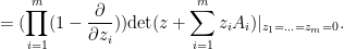
Proposition 3 (Deterministic multilinearisation formula) Let be the sum of deterministic rank one matrices . Then we have

for all , where the mixed characteristic polynomial of any matrices (not necessarily rank one) is given by the formula

Among other things, this formula gives a useful representation of the mean characteristic polynomial :

Corollary 4 (Random multilinearisation formula) Let be the sum of jointly independent rank one matrices . Then we have

for all .

Proof: For fixed , the expression is a polynomial combination of the , while the differential operator is a linear combination of differential operators for . As a consequence, we may expand (3) as a linear combination of terms, each of which is a multilinear combination of for some . Taking expectations of both sides of (2) and using the joint independence of the , we obtain the claim.

In view of Proposition 2, we can now hope to control the operator norm of certain special types of random matrices (and specifically, the sum of independent Hermitian positive semi-definite rank one matrices) by first controlling the mean of the random characteristic polynomial . Pursuing this philosophy, Marcus, Spielman, and Srivastava establish the following result, which they then use to prove the Kadison-Singer conjecture:

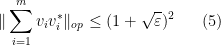
Theorem 5 (Marcus-Spielman-Srivastava theorem) Let . Let be jointly independent random vectors in , with each taking a finite number of values. Suppose that we have the normalisation

where we are using the convention that is the identity matrix whenever necessary. Suppose also that we have the smallness condition

for some and all . Then one has

with positive probability.

Note that the upper bound in (5) must be at least (by taking to be deterministic) and also must be at least (by taking the to always have magnitude at least ). Thus the bound in (5) is asymptotically tight both in the regime and in the regime ; the latter regime will be particularly useful for applications to Kadison-Singer. It should also be noted that if one uses more traditional random matrix theory methods (based on tools such as Proposition 1, as well as more sophisticated variants of these tools, such as the concentration of measure results of Rudelson and Ahlswede-Winter), one obtains a bound of with high probability, which is insufficient for the application to the Kadison-Singer problem; see this article of Tropp. Thus, Theorem 5 obtains a sharper bound, at the cost of trading in “high probability” for “positive probability”.

In the paper of Marcus, Spielman and Srivastava, Theorem 5 is used to deduce a conjecture of Weaver, which was already known to imply the Kadison-Singer conjecture; actually, a slight modification of their argument gives the paving conjecture of Kadison and Singer, from which the original Kadison-Singer conjecture may be readily deduced. We give these implications below the fold. (See also this survey article for some background on the Kadison-Singer problem.)

Let us now summarise how Theorem 5 is proven. In the spirit of semi-definite programming, we rephrase the above theorem in terms of the rank one Hermitian positive semi-definite matrices :

Theorem 6 (Marcus-Spielman-Srivastava theorem again) Let be jointly independent random rank one Hermitian positive semi-definite matrices such that the sum has mean

and such that

for some and all . Then one has

with positive probability.

In view of (1) and Proposition 2, this theorem follows from the following control on the mean characteristic polynomial:

Theorem 7 (Control of mean characteristic polynomial) Let be jointly independent random rank one Hermitian positive semi-definite matrices such that the sum has mean

and such that

for some and all . Then one has

This result is proven using the multilinearisation formula (Corollary 4) and some convexity properties of real stable polynomials; we give the proof below the fold.

Thanks to Adam Marcus, Assaf Naor and Sorin Popa for many useful explanations on various aspects of the Kadison-Singer problem.