You are currently browsing the monthly archive for November 2019.

Asgar Jamneshan and I have just uploaded to the arXiv our paper “An uncountable Moore-Schmidt theorem“. This paper revisits a classical theorem of Moore and Schmidt in measurable cohomology of measure-preserving systems. To state the theorem, let {X = (X,{\mathcal X},\mu)} be a probability space, and {\mathrm{Aut}(X, {\mathcal X}, \mu)} be the group of measure-preserving automorphisms of this space, that is to say the invertible bimeasurable maps {T: X \rightarrow X} that preserve the measure {\mu}: {T_* \mu = \mu}. To avoid some ambiguity later in this post when we introduce abstract analogues of measure theory, we will refer to measurable maps as concrete measurable maps, and measurable spaces as concrete measurable spaces. (One could also call {X = (X,{\mathcal X}, \mu)} a concrete probability space, but we will not need to do so here as we will not be working explicitly with abstract probability spaces.)

Let {\Gamma = (\Gamma,\cdot)} be a discrete group. A (concrete) measure-preserving action of {\Gamma} on {X} is a group homomorphism {\gamma \mapsto T^\gamma} from {\Gamma} to {\mathrm{Aut}(X, {\mathcal X}, \mu)}, thus {T^1} is the identity map and {T^{\gamma_1} \circ T^{\gamma_2} = T^{\gamma_1 \gamma_2}} for all {\gamma_1,\gamma_2 \in \Gamma}. A large portion of ergodic theory is concerned with the study of such measure-preserving actions, especially in the classical case when {\Gamma} is the integers (with the additive group law).

Let {K = (K,+)} be a compact Hausdorff abelian group, which we can endow with the Borel {\sigma}-algebra {{\mathcal B}(K)}. A (concrete measurable) {K}cocycle is a collection {\rho = (\rho_\gamma)_{\gamma \in \Gamma}} of concrete measurable maps {\rho_\gamma: X \rightarrow K} obeying the cocycle equation

\displaystyle \rho_{\gamma_1 \gamma_2}(x) = \rho_{\gamma_1} \circ T^{\gamma_2}(x) + \rho_{\gamma_2}(x) \ \ \ \ \ (1)

for {\mu}-almost every {x \in X}. (Here we are glossing over a measure-theoretic subtlety that we will return to later in this post – see if you can spot it before then!) Cocycles arise naturally in the theory of group extensions of dynamical systems; in particular (and ignoring the aforementioned subtlety), each cocycle induces a measure-preserving action {\gamma \mapsto S^\gamma} on {X \times K} (which we endow with the product of {\mu} with Haar probability measure on {K}), defined by

\displaystyle S^\gamma( x, k ) := (T^\gamma x, k + \rho_\gamma(x) ).

This connection with group extensions was the original motivation for our study of measurable cohomology, but is not the focus of the current paper.

A special case of a {K}-valued cocycle is a (concrete measurable) {K}-valued coboundary, in which {\rho_\gamma} for each {\gamma \in \Gamma} takes the special form

\displaystyle \rho_\gamma(x) = F \circ T^\gamma(x) - F(x)

for {\mu}-almost every {x \in X}, where {F: X \rightarrow K} is some measurable function; note that (ignoring the aforementioned subtlety), every function of this form is automatically a concrete measurable {K}-valued cocycle. One of the first basic questions in measurable cohomology is to try to characterize which {K}-valued cocycles are in fact {K}-valued coboundaries. This is a difficult question in general. However, there is a general result of Moore and Schmidt that at least allows one to reduce to the model case when {K} is the unit circle {\mathbf{T} = {\bf R}/{\bf Z}}, by taking advantage of the Pontryagin dual group {\hat K} of characters {\hat k: K \rightarrow \mathbf{T}}, that is to say the collection of continuous homomorphisms {\hat k: k \mapsto \langle \hat k, k \rangle} to the unit circle. More precisely, we have

Theorem 1 (Countable Moore-Schmidt theorem) Let {\Gamma} be a discrete group acting in a concrete measure-preserving fashion on a probability space {X}. Let {K} be a compact Hausdorff abelian group. Assume the following additional hypotheses:

Then a {K}-valued concrete measurable cocycle {\rho = (\rho_\gamma)_{\gamma \in \Gamma}} is a concrete coboundary if and only if for each character {\hat k \in \hat K}, the {\mathbf{T}}-valued cocycles {\langle \hat k, \rho \rangle = ( \langle \hat k, \rho_\gamma \rangle )_{\gamma \in \Gamma}} are concrete coboundaries.

The hypotheses (i), (ii), (iii) are saying in some sense that the data {\Gamma, X, K} are not too “large”; in all three cases they are saying in some sense that the data are only “countably complicated”. For instance, (iii) is equivalent to {K} being second countable, and (ii) is equivalent to {X} being modeled by a complete separable metric space. It is because of this restriction that we refer to this result as a “countable” Moore-Schmidt theorem. This theorem is a useful tool in several other applications, such as the Host-Kra structure theorem for ergodic systems; I hope to return to these subsequent applications in a future post.

Let us very briefly sketch the main ideas of the proof of Theorem 1. Ignore for now issues of measurability, and pretend that something that holds almost everywhere in fact holds everywhere. The hard direction is to show that if each {\langle \hat k, \rho \rangle} is a coboundary, then so is {\rho}. By hypothesis, we then have an equation of the form

\displaystyle \langle \hat k, \rho_\gamma(x) \rangle = \alpha_{\hat k} \circ T^\gamma(x) - \alpha_{\hat k}(x) \ \ \ \ \ (2)

for all {\hat k, \gamma, x} and some functions {\alpha_{\hat k}: X \rightarrow {\mathbf T}}, and our task is then to produce a function {F: X \rightarrow K} for which

\displaystyle \rho_\gamma(x) = F \circ T^\gamma(x) - F(x)

for all {\gamma,x}.

Comparing the two equations, the task would be easy if we could find an {F: X \rightarrow K} for which

\displaystyle \langle \hat k, F(x) \rangle = \alpha_{\hat k}(x) \ \ \ \ \ (3)

for all {\hat k, x}. However there is an obstruction to this: the left-hand side of (3) is additive in {\hat k}, so the right-hand side would have to be also in order to obtain such a representation. In other words, for this strategy to work, one would have to first establish the identity

\displaystyle \alpha_{\hat k_1 + \hat k_2}(x) - \alpha_{\hat k_1}(x) - \alpha_{\hat k_2}(x) = 0 \ \ \ \ \ (4)

for all {\hat k_1, \hat k_2, x}. On the other hand, the good news is that if we somehow manage to obtain the equation, then we can obtain a function {F} obeying (3), thanks to Pontryagin duality, which gives a one-to-one correspondence between {K} and the homomorphisms of the (discrete) group {\hat K} to {\mathbf{T}}.

Now, it turns out that one cannot derive the equation (4) directly from the given information (2). However, the left-hand side of (2) is additive in {\hat k}, so the right-hand side must be also. Manipulating this fact, we eventually arrive at

\displaystyle (\alpha_{\hat k_1 + \hat k_2} - \alpha_{\hat k_1} - \alpha_{\hat k_2}) \circ T^\gamma(x) = (\alpha_{\hat k_1 + \hat k_2} - \alpha_{\hat k_1} - \alpha_{\hat k_2})(x).

In other words, we don’t get to show that the left-hand side of (4) vanishes, but we do at least get to show that it is {\Gamma}-invariant. Now let us assume for sake of argument that the action of {\Gamma} is ergodic, which (ignoring issues about sets of measure zero) basically asserts that the only {\Gamma}-invariant functions are constant. So now we get a weaker version of (4), namely

\displaystyle \alpha_{\hat k_1 + \hat k_2}(x) - \alpha_{\hat k_1}(x) - \alpha_{\hat k_2}(x) = c_{\hat k_1, \hat k_2} \ \ \ \ \ (5)

for some constants {c_{\hat k_1, \hat k_2} \in \mathbf{T}}.

Now we need to eliminate the constants. This can be done by the following group-theoretic projection. Let {L^0({\bf X} \rightarrow {\bf T})} denote the space of concrete measurable maps {\alpha} from {{\bf X}} to {{\bf T}}, up to almost everywhere equivalence; this is an abelian group where the various terms in (5) naturally live. Inside this group we have the subgroup {{\bf T}} of constant functions (up to almost everywhere equivalence); this is where the right-hand side of (5) lives. Because {{\bf T}} is a divisible group, there is an application of Zorn’s lemma (a good exercise for those who are not acquainted with these things) to show that there exists a retraction {w: L^0({\bf X} \rightarrow {\bf T}) \rightarrow {\bf T}}, that is to say a group homomorphism that is the identity on the subgroup {{\bf T}}. We can use this retraction, or more precisely the complement {\alpha \mapsto \alpha - w(\alpha)}, to eliminate the constant in (5). Indeed, if we set

\displaystyle \tilde \alpha_{\hat k}(x) := \alpha_{\hat k}(x) - w(\alpha_{\hat k})

then from (5) we see that

\displaystyle \tilde \alpha_{\hat k_1 + \hat k_2}(x) - \tilde \alpha_{\hat k_1}(x) - \tilde \alpha_{\hat k_2}(x) = 0

while from (2) one has

\displaystyle \langle \hat k, \rho_\gamma(x) \rangle = \tilde \alpha_{\hat k} \circ T^\gamma(x) - \tilde \alpha_{\hat k}(x)

and now the previous strategy works with {\alpha_{\hat k}} replaced by {\tilde \alpha_{\hat k}}. This concludes the sketch of proof of Theorem 1.

In making the above argument rigorous, the hypotheses (i)-(iii) are used in several places. For instance, to reduce to the ergodic case one relies on the ergodic decomposition, which requires the hypothesis (ii). Also, most of the above equations only hold outside of a set of measure zero, and the hypothesis (i) and the hypothesis (iii) (which is equivalent to {\hat K} being at most countable) to avoid the problem that an uncountable union of sets of measure zero could have positive measure (or fail to be measurable at all).

My co-author Asgar Jamneshan and I are working on a long-term project to extend many results in ergodic theory (such as the aforementioned Host-Kra structure theorem) to “uncountable” settings in which hypotheses analogous to (i)-(iii) are omitted; thus we wish to consider actions on uncountable groups, on spaces that are not standard Borel, and cocycles taking values in groups that are not metrisable. Such uncountable contexts naturally arise when trying to apply ergodic theory techniques to combinatorial problems (such as the inverse conjecture for the Gowers norms), as one often relies on the ultraproduct construction (or something similar) to generate an ergodic theory translation of these problems, and these constructions usually give “uncountable” objects rather than “countable” ones. (For instance, the ultraproduct of finite groups is a hyperfinite group, which is usually uncountable.). This paper marks the first step in this project by extending the Moore-Schmidt theorem to the uncountable setting.

If one simply drops the hypotheses (i)-(iii) and tries to prove the Moore-Schmidt theorem, several serious difficulties arise. We have already mentioned the loss of the ergodic decomposition and the possibility that one has to control an uncountable union of null sets. But there is in fact a more basic problem when one deletes (iii): the addition operation {+: K \times K \rightarrow K}, while still continuous, can fail to be measurable as a map from {(K \times K, {\mathcal B}(K) \otimes {\mathcal B}(K))} to {(K, {\mathcal B}(K))}! Thus for instance the sum of two measurable functions {F: X \rightarrow K} need not remain measurable, which makes even the very definition of a measurable cocycle or measurable coboundary problematic (or at least unnatural). This phenomenon is known as the Nedoma pathology. A standard example arises when {K} is the uncountable torus {{\mathbf T}^{{\bf R}}}, endowed with the product topology. Crucially, the Borel {\sigma}-algebra {{\mathcal B}(K)} generated by this uncountable product is not the product {{\mathcal B}(\mathbf{T})^{\otimes {\bf R}}} of the factor Borel {\sigma}-algebras (the discrepancy ultimately arises from the fact that topologies permit uncountable unions, but {\sigma}-algebras do not); relating to this, the product {\sigma}-algebra {{\mathcal B}(K) \otimes {\mathcal B}(K)} is not the same as the Borel {\sigma}-algebra {{\mathcal B}(K \times K)}, but is instead a strict sub-algebra. If the group operations on {K} were measurable, then the diagonal set

\displaystyle K^\Delta := \{ (k,k') \in K \times K: k = k' \} = \{ (k,k') \in K \times K: k - k' = 0 \}

would be measurable in {{\mathcal B}(K) \otimes {\mathcal B}(K)}. But it is an easy exercise in manipulation of {\sigma}-algebras to show that if {(X, {\mathcal X}), (Y, {\mathcal Y})} are any two measurable spaces and {E \subset X \times Y} is measurable in {{\mathcal X} \otimes {\mathcal Y}}, then the fibres {E_x := \{ y \in Y: (x,y) \in E \}} of {E} are contained in some countably generated subalgebra of {{\mathcal Y}}. Thus if {K^\Delta} were {{\mathcal B}(K) \otimes {\mathcal B}(K)}-measurable, then all the points of {K} would lie in a single countably generated {\sigma}-algebra. But the cardinality of such an algebra is at most {2^{\alpha_0}} while the cardinality of {K} is {2^{2^{\alpha_0}}}, and Cantor’s theorem then gives a contradiction.

To resolve this problem, we give {K} a coarser {\sigma}-algebra than the Borel {\sigma}-algebra, namely the Baire {\sigma}-algebra {{\mathcal B}^\otimes(K)}, thus coarsening the measurable space structure on {K = (K,{\mathcal B}(K))} to a new measurable space {K_\otimes := (K, {\mathcal B}^\otimes(K))}. In the case of compact Hausdorff abelian groups, {{\mathcal B}^{\otimes}(K)} can be defined as the {\sigma}-algebra generated by the characters {\hat k: K \rightarrow {\mathbf T}}; for more general compact abelian groups, one can define {{\mathcal B}^{\otimes}(K)} as the {\sigma}-algebra generated by all continuous maps into metric spaces. This {\sigma}-algebra is equal to {{\mathcal B}(K)} when {K} is metrisable but can be smaller for other {K}. With this measurable structure, {K_\otimes} becomes a measurable group; it seems that once one leaves the metrisable world that {K_\otimes} is a superior (or at least equally good) space to work with than {K} for analysis, as it avoids the Nedoma pathology. (For instance, from Plancherel’s theorem, we see that if {m_K} is the Haar probability measure on {K}, then {L^2(K,m_K) = L^2(K_\otimes,m_K)} (thus, every {K}-measurable set is equivalent modulo {m_K}-null sets to a {K_\otimes}-measurable set), so there is no damage to Plancherel caused by passing to the Baire {\sigma}-algebra.

Passing to the Baire {\sigma}-algebra {K_\otimes} fixes the most severe problems with an uncountable Moore-Schmidt theorem, but one is still faced with an issue of having to potentially take an uncountable union of null sets. To avoid this sort of problem, we pass to the framework of abstract measure theory, in which we remove explicit mention of “points” and can easily delete all null sets at a very early stage of the formalism. In this setup, the category of concrete measurable spaces is replaced with the larger category of abstract measurable spaces, which we formally define as the opposite category of the category of {\sigma}-algebras (with Boolean algebra homomorphisms). Thus, we define an abstract measurable space to be an object of the form {{\mathcal X}^{\mathrm{op}}}, where {{\mathcal X}} is an (abstract) {\sigma}-algebra and {\mathrm{op}} is a formal placeholder symbol that signifies use of the opposite category, and an abstract measurable map {T: {\mathcal X}^{\mathrm{op}} \rightarrow {\mathcal Y}^{\mathrm{op}}} is an object of the form {(T^*)^{\mathrm{op}}}, where {T^*: {\mathcal Y} \rightarrow {\mathcal X}} is a Boolean algebra homomorphism and {\mathrm{op}} is again used as a formal placeholder; we call {T^*} the pullback map associated to {T}.  [UPDATE: It turns out that this definition of a measurable map led to technical issues.  In a forthcoming revision of the paper we also impose the requirement that the abstract measurable map be \sigma-complete (i.e., it respects countable joins).] The composition {S \circ T: {\mathcal X}^{\mathrm{op}} \rightarrow {\mathcal Z}^{\mathrm{op}}} of two abstract measurable maps {T: {\mathcal X}^{\mathrm{op}} \rightarrow {\mathcal Y}^{\mathrm{op}}}, {S: {\mathcal Y}^{\mathrm{op}} \rightarrow {\mathcal Z}^{\mathrm{op}}} is defined by the formula {S \circ T := (T^* \circ S^*)^{\mathrm{op}}}, or equivalently {(S \circ T)^* = T^* \circ S^*}.

Every concrete measurable space {X = (X,{\mathcal X})} can be identified with an abstract counterpart {{\mathcal X}^{op}}, and similarly every concrete measurable map {T: X \rightarrow Y} can be identified with an abstract counterpart {(T^*)^{op}}, where {T^*: {\mathcal Y} \rightarrow {\mathcal X}} is the pullback map {T^* E := T^{-1}(E)}. Thus the category of concrete measurable spaces can be viewed as a subcategory of the category of abstract measurable spaces. The advantage of working in the abstract setting is that it gives us access to more spaces that could not be directly defined in the concrete setting. Most importantly for us, we have a new abstract space, the opposite measure algebra {X_\mu} of {X}, defined as {({\bf X}/{\bf N})^*} where {{\bf N}} is the ideal of null sets in {{\bf X}}. Informally, {X_\mu} is the space {X} with all the null sets removed; there is a canonical abstract embedding map {\iota: X_\mu \rightarrow X}, which allows one to convert any concrete measurable map {f: X \rightarrow Y} into an abstract one {[f]: X_\mu \rightarrow Y}. One can then define the notion of an abstract action, abstract cocycle, and abstract coboundary by replacing every occurrence of the category of concrete measurable spaces with their abstract counterparts, and replacing {X} with the opposite measure algebra {X_\mu}; see the paper for details. Our main theorem is then

Theorem 2 (Uncountable Moore-Schmidt theorem) Let {\Gamma} be a discrete group acting abstractly on a {\sigma}-finite measure space {X}. Let {K} be a compact Hausdorff abelian group. Then a {K_\otimes}-valued abstract measurable cocycle {\rho = (\rho_\gamma)_{\gamma \in \Gamma}} is an abstract coboundary if and only if for each character {\hat k \in \hat K}, the {\mathbf{T}}-valued cocycles {\langle \hat k, \rho \rangle = ( \langle \hat k, \rho_\gamma \rangle )_{\gamma \in \Gamma}} are abstract coboundaries.

With the abstract formalism, the proof of the uncountable Moore-Schmidt theorem is almost identical to the countable one (in fact we were able to make some simplifications, such as avoiding the use of the ergodic decomposition). A key tool is what we call a “conditional Pontryagin duality” theorem, which asserts that if one has an abstract measurable map {\alpha_{\hat k}: X_\mu \rightarrow {\bf T}} for each {\hat k \in K} obeying the identity { \alpha_{\hat k_1 + \hat k_2} - \alpha_{\hat k_1} - \alpha_{\hat k_2} = 0} for all {\hat k_1,\hat k_2 \in \hat K}, then there is an abstract measurable map {F: X_\mu \rightarrow K_\otimes} such that {\alpha_{\hat k} = \langle \hat k, F \rangle} for all {\hat k \in \hat K}. This is derived from the usual Pontryagin duality and some other tools, most notably the completeness of the {\sigma}-algebra of {X_\mu}, and the Sikorski extension theorem.

We feel that it is natural to stay within the abstract measure theory formalism whenever dealing with uncountable situations. However, it is still an interesting question as to when one can guarantee that the abstract objects constructed in this formalism are representable by concrete analogues. The basic questions in this regard are:

  • (i) Suppose one has an abstract measurable map {f: X_\mu \rightarrow Y} into a concrete measurable space. Does there exist a representation of {f} by a concrete measurable map {\tilde f: X \rightarrow Y}? Is it unique up to almost everywhere equivalence?
  • (ii) Suppose one has a concrete cocycle that is an abstract coboundary. When can it be represented by a concrete coboundary?

For (i) the answer is somewhat interesting (as I learned after posing this MathOverflow question):

  • If {Y} does not separate points, or is not compact metrisable or Polish, there can be counterexamples to uniqueness. If {Y} is not compact or Polish, there can be counterexamples to existence.
  • If {Y} is a compact metric space or a Polish space, then one always has existence and uniqueness.
  • If {Y} is a compact Hausdorff abelian group, one always has existence.
  • If {X} is a complete measure space, then one always has existence (from a theorem of Maharam).
  • If {X} is the unit interval with the Borel {\sigma}-algebra and Lebesgue measure, then one has existence for all compact Hausdorff {Y} assuming the continuum hypothesis (from a theorem of von Neumann) but existence can fail under other extensions of ZFC (from a theorem of Shelah, using the method of forcing).
  • For more general {X}, existence for all compact Hausdorff {Y} is equivalent to the existence of a lifting from the {\sigma}-algebra {\mathcal{X}/\mathcal{N}} to {\mathcal{X}} (or, in the language of abstract measurable spaces, the existence of an abstract retraction from {X} to {X_\mu}).
  • It is a long-standing open question (posed for instance by Fremlin) whether it is relatively consistent with ZFC that existence holds whenever {Y} is compact Hausdorff.

Our understanding of (ii) is much less complete:

  • If {K} is metrisable, the answer is “always” (which among other things establishes the countable Moore-Schmidt theorem as a corollary of the uncountable one).
  • If {\Gamma} is at most countable and {X} is a complete measure space, then the answer is again “always”.

In view of the answers to (i), I would not be surprised if the full answer to (ii) was also sensitive to axioms of set theory. However, such set theoretic issues seem to be almost completely avoided if one sticks with the abstract formalism throughout; they only arise when trying to pass back and forth between the abstract and concrete categories.

In these notes we presume familiarity with the basic concepts of probability theory, such as random variables (which could take values in the reals, vectors, or other measurable spaces), probability, and expectation. Much of this theory is in turn based on measure theory, which we will also presume familiarity with. See for instance this previous set of lecture notes for a brief review.

The basic objects of study in analytic number theory are deterministic; there is nothing inherently random about the set of prime numbers, for instance. Despite this, one can still interpret many of the averages encountered in analytic number theory in probabilistic terms, by introducing random variables into the subject. Consider for instance the form

\displaystyle \sum_{n \leq x} \mu(n) = o(x) \ \ \ \ \ (1)


of the prime number theorem (where we take the limit {x \rightarrow \infty}). One can interpret this estimate probabilistically as

\displaystyle {\mathbb E} \mu(\mathbf{n}) = o(1) \ \ \ \ \ (2)

where {\mathbf{n} = \mathbf{n}_{\leq x}} is a random variable drawn uniformly from the natural numbers up to {x}, and {{\mathbb E}} denotes the expectation. (In this set of notes we will use boldface symbols to denote random variables, and non-boldface symbols for deterministic objects.) By itself, such an interpretation is little more than a change of notation. However, the power of this interpretation becomes more apparent when one then imports concepts from probability theory (together with all their attendant intuitions and tools), such as independence, conditioning, stationarity, total variation distance, and entropy. For instance, suppose we want to use the prime number theorem (1) to make a prediction for the sum

\displaystyle \sum_{n \leq x} \mu(n) \mu(n+1).

After dividing by {x}, this is essentially

\displaystyle {\mathbb E} \mu(\mathbf{n}) \mu(\mathbf{n}+1).

With probabilistic intuition, one may expect the random variables {\mu(\mathbf{n}), \mu(\mathbf{n}+1)} to be approximately independent (there is no obvious relationship between the number of prime factors of {\mathbf{n}}, and of {\mathbf{n}+1}), and so the above average would be expected to be approximately equal to

\displaystyle ({\mathbb E} \mu(\mathbf{n})) ({\mathbb E} \mu(\mathbf{n}+1))

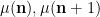
which by (2) is equal to {o(1)}. Thus we are led to the prediction

\displaystyle \sum_{n \leq x} \mu(n) \mu(n+1) = o(x). \ \ \ \ \ (3)

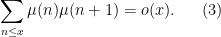
The asymptotic (3) is widely believed (it is a special case of the Chowla conjecture, which we will discuss in later notes; while there has been recent progress towards establishing it rigorously, it remains open for now.
How would one try to make these probabilistic intuitions more rigorous? The first thing one needs to do is find a more quantitative measurement of what it means for two random variables to be “approximately” independent. There are several candidates for such measurements, but we will focus in these notes on two particularly convenient measures of approximate independence: the “{L^2}” measure of independence known as covariance, and the “{L \log L}” measure of independence known as mutual information (actually we will usually need the more general notion of conditional mutual information that measures conditional independence). The use of {L^2} type methods in analytic number theory is well established, though it is usually not described in probabilistic terms, being referred to instead by such names as the “second moment method”, the “large sieve” or the “method of bilinear sums”. The use of {L \log L} methods (or “entropy methods”) is much more recent, and has been able to control certain types of averages in analytic number theory that were out of reach of previous methods such as {L^2} methods. For instance, in later notes we will use entropy methods to establish the logarithmically averaged version

\displaystyle \sum_{n \leq x} \frac{\mu(n) \mu(n+1)}{n} = o(\log x) \ \ \ \ \ (4)


of (3), which is implied by (3) but strictly weaker (much as the prime number theorem (1) implies the bound {\sum_{n \leq x} \frac{\mu(n)}{n} = o(\log x)}, but the latter bound is much easier to establish than the former).
As with many other situations in analytic number theory, we can exploit the fact that certain assertions (such as approximate independence) can become significantly easier to prove if one only seeks to establish them on average, rather than uniformly. For instance, given two random variables {\mathbf{X}} and {\mathbf{Y}} of number-theoretic origin (such as the random variables {\mu(\mathbf{n})} and {\mu(\mathbf{n}+1)} mentioned previously), it can often be extremely difficult to determine the extent to which {\mathbf{X},\mathbf{Y}} behave “independently” (or “conditionally independently”). However, thanks to second moment tools or entropy based tools, it is often possible to assert results of the following flavour: if {\mathbf{Y}_1,\dots,\mathbf{Y}_k} are a large collection of “independent” random variables, and {\mathbf{X}} is a further random variable that is “not too large” in some sense, then {\mathbf{X}} must necessarily be nearly independent (or conditionally independent) to many of the {\mathbf{Y}_i}, even if one cannot pinpoint precisely which of the {\mathbf{Y}_i} the variable {\mathbf{X}} is independent with. In the case of the second moment method, this allows us to compute correlations such as {{\mathbb E} {\mathbf X} \mathbf{Y}_i} for “most” {i}. The entropy method gives bounds that are significantly weaker quantitatively than the second moment method (and in particular, in its current incarnation at least it is only able to say non-trivial assertions involving interactions with residue classes at small primes), but can control significantly more general quantities {{\mathbb E} F( {\mathbf X}, \mathbf{Y}_i )} for “most” {i} thanks to tools such as the Pinsker inequality.

Read the rest of this entry »

Archives