You are currently browsing the monthly archive for August 2019.

William Banks, Kevin Ford, and I have just uploaded to the arXiv our paper “Large prime gaps and probabilistic models“. In this paper we introduce a random model to help understand the connection between two well known conjectures regarding the primes {{\mathcal P} := \{2,3,5,\dots\}}, the Cramér conjecture and the Hardy-Littlewood conjecture:

Conjecture 1 (Cramér conjecture) If {x} is a large number, then the largest prime gap {G_{\mathcal P}(x) := \sup_{p_n, p_{n+1} \leq x} p_{n+1}-p_n} in {[1,x]} is of size {\asymp \log^2 x}. (Granville refines this conjecture to {\gtrsim \xi \log^2 x}, where {\xi := 2e^{-\gamma} = 1.1229\dots}. Here we use the asymptotic notation {X \gtrsim Y} for {X \geq (1-o(1)) Y}, {X \sim Y} for {X \gtrsim Y \gtrsim X}, {X \gg Y} for {X \geq C^{-1} Y}, and {X \asymp Y} for {X \gg Y \gg X}.)

Conjecture 2 (Hardy-Littlewood conjecture) If {\mathcal{H} := \{h_1,\dots,h_k\}} are fixed distinct integers, then the number of numbers {n \in [1,x]} with {n+h_1,\dots,n+h_k} all prime is {({\mathfrak S}(\mathcal{H}) +o(1)) \int_2^x \frac{dt}{\log^k t}} as {x \rightarrow \infty}, where the singular series {{\mathfrak S}(\mathcal{H})} is defined by the formula

\displaystyle {\mathfrak S}(\mathcal{H}) := \prod_p \left( 1 - \frac{|{\mathcal H} \hbox{ mod } p|}{p}\right) (1-\frac{1}{p})^{-k}.

(One can view these conjectures as modern versions of two of the classical Landau problems, namely Legendre’s conjecture and the twin prime conjecture respectively.)

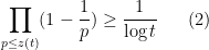
A well known connection between the Hardy-Littlewood conjecture and prime gaps was made by Gallagher. Among other things, Gallagher showed that if the Hardy-Littlewood conjecture was true, then the prime gaps {p_{n+1}-p_n} with {n \leq x} were asymptotically distributed according to an exponential distribution of mean {\log x}, in the sense that

\displaystyle | \{ n: p_n \leq x, p_{n+1}-p_n \geq \lambda \log x \}| = (e^{-\lambda}+o(1)) \frac{x}{\log x} \ \ \ \ \ (1)


as {x \rightarrow \infty} for any fixed {\lambda \geq 0}. Roughly speaking, the way this is established is by using the Hardy-Littlewood conjecture to control the mean values of {\binom{|{\mathcal P} \cap (p_n, p_n + \lambda \log x)|}{k}} for fixed {k,\lambda}, where {p_n} ranges over the primes in {[1,x]}. The relevance of these quantities arises from the Bonferroni inequalities (or “Brun pure sieve“), which can be formulated as the assertion that

\displaystyle 1_{N=0} \leq \sum_{k=0}^K (-1)^k \binom{N}{k}

when {K} is even and

\displaystyle 1_{N=0} \geq \sum_{k=0}^K (-1)^k \binom{N}{k}

when {K} is odd, for any natural number {N}; setting {N := |{\mathcal P} \cap (p_n, p_n + \lambda \log x)|} and taking means, one then gets upper and lower bounds for the probability that the interval {(p_n, p_n + \lambda \log x)} is free of primes. The most difficult step is to control the mean values of the singular series {{\mathfrak S}(\mathcal{H})} as {{\mathcal H}} ranges over {k}-tuples in a fixed interval such as {[0, \lambda \log x]}.

Heuristically, if one extrapolates the asymptotic (1) to the regime {\lambda \asymp \log x}, one is then led to Cramér’s conjecture, since the right-hand side of (1) falls below {1} when {\lambda} is significantly larger than {\log x}. However, this is not a rigorous derivation of Cramér’s conjecture from the Hardy-Littlewood conjecture, since Gallagher’s computations only establish (1) for fixed choices of {\lambda}, which is only enough to establish the far weaker bound {G_{\mathcal P}(x) / \log x \rightarrow \infty}, which was already known (see this previous paper for a discussion of the best known unconditional lower bounds on {G_{\mathcal P}(x)}). An inspection of the argument shows that if one wished to extend (1) to parameter choices {\lambda} that were allowed to grow with {x}, then one would need as input a stronger version of the Hardy-Littlewood conjecture in which the length {k} of the tuple {{\mathcal H} = (h_1,\dots,h_k)}, as well as the magnitudes of the shifts {h_1,\dots,h_k}, were also allowed to grow with {x}. Our initial objective in this project was then to quantify exactly what strengthening of the Hardy-Littlewood conjecture would be needed to rigorously imply Cramer’s conjecture. The precise results are technical, but roughly we show results of the following form:

Theorem 3 (Large gaps from Hardy-Littlewood, rough statement)

  • If the Hardy-Littlewood conjecture is uniformly true for {k}-tuples of length {k \ll \frac{\log x}{\log\log x}}, and with shifts {h_1,\dots,h_k} of size {O( \log^2 x )}, with a power savings in the error term, then {G_{\mathcal P}(x) \gg \frac{\log^2 x}{\log\log x}}.
  • If the Hardy-Littlewood conjecture is “true on average” for {k}-tuples of length {k \ll \frac{y}{\log x}} and shifts {h_1,\dots,h_k} of size {y} for all {\log x \leq y \leq \log^2 x \log\log x}, with a power savings in the error term, then {G_{\mathcal P}(x) \gg \log^2 x}.

In particular, we can recover Cramer’s conjecture given a sufficiently powerful version of the Hardy-Littlewood conjecture “on the average”.

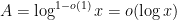
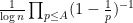
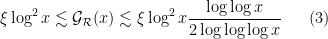
Our proof of this theorem proceeds more or less along the same lines as Gallagher’s calculation, but now with {k} allowed to grow slowly with {x}. Again, the main difficulty is to accurately estimate average values of the singular series {{\mathfrak S}({\mathfrak H})}. Here we found it useful to switch to a probabilistic interpretation of this series. For technical reasons it is convenient to work with a truncated, unnormalised version

\displaystyle V_{\mathcal H}(z) := \prod_{p \leq z} \left( 1 - \frac{|{\mathcal H} \hbox{ mod } p|}{p} \right)

of the singular series, for a suitable cutoff {z}; it turns out that when studying prime tuples of size {t}, the most convenient cutoff {z(t)} is the “Pólya magic cutoff“, defined as the largest prime for which

\displaystyle \prod_{p \leq z(t)}(1-\frac{1}{p}) \geq \frac{1}{\log t} \ \ \ \ \ (2)


(this is well defined for {t \geq e^2}); by Mertens’ theorem, we have {z(t) \sim t^{1/e^\gamma}}. One can interpret {V_{\mathcal Z}(z)} probabilistically as

\displaystyle V_{\mathcal Z}(z) = \mathbf{P}( {\mathcal H} \subset \mathcal{S}_z )

where {\mathcal{S}_z \subset {\bf Z}} is the randomly sifted set of integers formed by removing one residue class {a_p \hbox{ mod } p} uniformly at random for each prime {p \leq z}. The Hardy-Littlewood conjecture can be viewed as an assertion that the primes {{\mathcal P}} behave in some approximate statistical sense like the random sifted set {\mathcal{S}_z}, and one can prove the above theorem by using the Bonferroni inequalities both for the primes {{\mathcal P}} and for the random sifted set, and comparing the two (using an even {K} for the sifted set and an odd {K} for the primes in order to be able to combine the two together to get a useful bound).

The proof of Theorem 3 ended up not using any properties of the set of primes {{\mathcal P}} other than that this set obeyed some form of the Hardy-Littlewood conjectures; the theorem remains true (with suitable notational changes) if this set were replaced by any other set. In order to convince ourselves that our theorem was not vacuous due to our version of the Hardy-Littlewood conjecture being too strong to be true, we then started exploring the question of coming up with random models of {{\mathcal P}} which obeyed various versions of the Hardy-Littlewood and Cramér conjectures.

This line of inquiry was started by Cramér, who introduced what we now call the Cramér random model {{\mathcal C}} of the primes, in which each natural number {n \geq 3} is selected for membership in {{\mathcal C}} with an independent probability of {1/\log n}. This model matches the primes well in some respects; for instance, it almost surely obeys the “Riemann hypothesis”

\displaystyle | {\mathcal C} \cap [1,x] | = \int_2^x \frac{dt}{\log t} + O( x^{1/2+o(1)})

and Cramér also showed that the largest gap {G_{\mathcal C}(x)} was almost surely {\sim \log^2 x}. On the other hand, it does not obey the Hardy-Littlewood conjecture; more precisely, it obeys a simplified variant of that conjecture in which the singular series {{\mathfrak S}({\mathcal H})} is absent.

Granville proposed a refinement {{\mathcal G}} to Cramér’s random model {{\mathcal C}} in which one first sieves out (in each dyadic interval {[x,2x]}) all residue classes {0 \hbox{ mod } p} for {p \leq A} for a certain threshold {A = \log^{1-o(1)} x = o(\log x)}, and then places each surviving natural number {n} in {{\mathcal G}} with an independent probability {\frac{1}{\log n} \prod_{p \leq A} (1-\frac{1}{p})^{-1}}. One can verify that this model obeys the Hardy-Littlewood conjectures, and Granville showed that the largest gap {G_{\mathcal G}(x)} in this model was almost surely {\gtrsim \xi \log^2 x}, leading to his conjecture that this bound also was true for the primes. (Interestingly, this conjecture is not yet borne out by numerics; calculations of prime gaps up to {10^{18}}, for instance, have shown that {G_{\mathcal P}(x)} never exceeds {0.9206 \log^2 x} in this range. This is not necessarily a conflict, however; Granville’s analysis relies on inspecting gaps in an extremely sparse region of natural numbers that are more devoid of primes than average, and this region is not well explored by existing numerics. See this previous blog post for more discussion of Granville’s argument.)

However, Granville’s model does not produce a power savings in the error term of the Hardy-Littlewood conjectures, mostly due to the need to truncate the singular series at the logarithmic cutoff {A}. After some experimentation, we were able to produce a tractable random model {{\mathcal R}} for the primes which obeyed the Hardy-Littlewood conjectures with power savings, and which reproduced Granville’s gap prediction of {\gtrsim \xi \log^2 x} (we also get an upper bound of {\lesssim \xi \log^2 x \frac{\log\log x}{2 \log\log\log x}} for both models, though we expect the lower bound to be closer to the truth); to us, this strengthens the case for Granville’s version of Cramér’s conjecture. The model can be described as follows. We select one residue class {a_p \hbox{ mod } p} uniformly at random for each prime {p}, and as before we let {S_z} be the sifted set of integers formed by deleting the residue classes {a_p \hbox{ mod } p} with {p \leq z}. We then set

\displaystyle {\mathcal R} := \{ n \geq e^2: n \in S_{z(t)}\}

with {z(t)} Pólya’s magic cutoff (this is the cutoff that gives {{\mathcal R}} a density consistent with the prime number theorem or the Riemann hypothesis). As stated above, we are able to show that almost surely one has

\displaystyle \xi \log^2 x \lesssim {\mathcal G}_{\mathcal R}(x) \lesssim \xi \log^2 x \frac{\log\log x}{2 \log\log\log x} \ \ \ \ \ (3)


and that the Hardy-Littlewood conjectures hold with power savings for {k} up to {\log^c x} for any fixed {c < 1} and for shifts {h_1,\dots,h_k} of size {O(\log^c x)}. This is unfortunately a tiny bit weaker than what Theorem 3 requires (which more or less corresponds to the endpoint {c=1}), although there is a variant of Theorem 3 that can use this input to produce a lower bound on gaps in the model {{\mathcal R}} (but it is weaker than the one in (3)). In fact we prove a more precise almost sure asymptotic formula for {{\mathcal G}_{\mathcal R}(x) } that involves the optimal bounds for the linear sieve (or interval sieve), in which one deletes one residue class modulo {p} from an interval {[0,y]} for all primes {p} up to a given threshold. The lower bound in (3) relates to the case of deleting the {0 \hbox{ mod } p} residue classes from {[0,y]}; the upper bound comes from the delicate analysis of the linear sieve by Iwaniec. Improving on either of the two bounds looks to be quite a difficult problem.

The probabilistic analysis of {{\mathcal R}} is somewhat more complicated than of {{\mathcal C}} or {{\mathcal G}} as there is now non-trivial coupling between the events {n \in {\mathcal R}} as {n} varies, although moment methods such as the second moment method are still viable and allow one to verify the Hardy-Littlewood conjectures by a lengthy but fairly straightforward calculation. To analyse large gaps, one has to understand the statistical behaviour of a random linear sieve in which one starts with an interval {[0,y]} and randomly deletes a residue class {a_p \hbox{ mod } p} for each prime {p} up to a given threshold. For very small {p} this is handled by the deterministic theory of the linear sieve as discussed above. For medium sized {p}, it turns out that there is good concentration of measure thanks to tools such as Bennett’s inequality or Azuma’s inequality, as one can view the sieving process as a martingale or (approximately) as a sum of independent random variables. For larger primes {p}, in which only a small number of survivors are expected to be sieved out by each residue class, a direct combinatorial calculation of all possible outcomes (involving the random graph that connects interval elements {n \in [0,y]} to primes {p} if {n} falls in the random residue class {a_p \hbox{ mod } p}) turns out to give the best results.

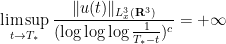
I’ve just uploaded to the arXiv my paper “Quantitative bounds for critically bounded solutions to the Navier-Stokes equations“, submitted to the proceedings of the Linde Hall Inaugural Math Symposium. (I unfortunately had to cancel my physical attendance at this symposium for personal reasons, but was still able to contribute to the proceedings.) In recent years I have been interested in working towards establishing the existence of classical solutions for the Navier-Stokes equations

\displaystyle \partial_t u + (u \cdot \nabla) u = \Delta u - \nabla p

\displaystyle \nabla \cdot u = 0

that blow up in finite time, but this time for a change I took a look at the other side of the theory, namely the conditional regularity results for this equation. There are several such results that assert that if a certain norm of the solution stays bounded (or grows at a controlled rate), then the solution stays regular; taken in the contrapositive, they assert that if a solution blows up at a certain finite time {T_*}, then certain norms of the solution must also go to infinity. Here are some examples (not an exhaustive list) of such blowup criteria:

  • (Leray blowup criterion, 1934) If {u} blows up at a finite time {T_*}, and {3 < p \leq \infty}, then {\liminf_{t \rightarrow T_*} (T_* - t)^{\frac{1}{2}-\frac{3}{2p}} \| u(t) \|_{L^p_x({\bf R}^3)} \geq c} for an absolute constant {c>0}.
  • (ProdiSerrinLadyzhenskaya blowup criterion, 1959-1967) If {u} blows up at a finite time {T_*}, and {3 < p \leq \infty}, then {\| u \|_{L^q_t L^p_x([0,T_*) \times {\bf R}^3)} =+\infty}, where {\frac{1}{q} := \frac{1}{2} - \frac{3}{2p}}.
  • (Beale-Kato-Majda blowup criterion, 1984) If {u} blows up at a finite time {T_*}, then {\| \omega \|_{L^1_t L^\infty_x([0,T_*) \times {\bf R}^3)} = +\infty}, where {\omega := \nabla \times u} is the vorticity.
  • (Kato blowup criterion, 1984) If {u} blows up at a finite time {T_*}, then {\liminf_{t \rightarrow T_*} \|u(t) \|_{L^3_x({\bf R}^3)} \geq c} for some absolute constant {c>0}.
  • (Escauriaza-Seregin-Sverak blowup criterion, 2003) If {u} blows up at a finite time {T_*}, then {\limsup_{t \rightarrow T_*} \|u(t) \|_{L^3_x({\bf R}^3)} = +\infty}.
  • (Seregin blowup criterion, 2012) If {u} blows up at a finite time {T_*}, then {\lim_{t \rightarrow T_*} \|u(t) \|_{L^3_x({\bf R}^3)} = +\infty}.
  • (Phuc blowup criterion, 2015) If {u} blows up at a finite time {T_*}, then {\limsup_{t \rightarrow T_*} \|u(t) \|_{L^{3,q}_x({\bf R}^3)} = +\infty} for any {q < \infty}.
  • (Gallagher-Koch-Planchon blowup criterion, 2016) If {u} blows up at a finite time {T_*}, then {\limsup_{t \rightarrow T_*} \|u(t) \|_{\dot B_{p,q}^{-1+3/p}({\bf R}^3)} = +\infty} for any {3 < p, q < \infty}.
  • (Albritton blowup criterion, 2016) If {u} blows up at a finite time {T_*}, then {\lim_{t \rightarrow T_*} \|u(t) \|_{\dot B_{p,q}^{-1+3/p}({\bf R}^3)} = +\infty} for any {3 < p, q < \infty}.

My current paper is most closely related to the Escauriaza-Seregin-Sverak blowup criterion, which was the first to show a critical (i.e., scale-invariant, or dimensionless) spatial norm, namely {L^3_x({\bf R}^3)}, had to become large. This result now has many proofs; for instance, many of the subsequent blowup criterion results imply the Escauriaza-Seregin-Sverak one as a special case, and there are also additional proofs by Gallagher-Koch-Planchon (building on ideas of Kenig-Koch), and by Dong-Du. However, all of these proofs rely on some form of a compactness argument: given a finite time blowup, one extracts some suitable family of rescaled solutions that converges in some weak sense to a limiting solution that has some additional good properties (such as almost periodicity modulo symmetries), which one can then rule out using additional qualitative tools, such as unique continuation and backwards uniqueness theorems for parabolic heat equations. In particular, all known proofs use some version of the backwards uniqueness theorem of Escauriaza, Seregin, and Sverak. Because of this reliance on compactness, the existing proofs of the Escauriaza-Seregin-Sverak blowup criterion are qualitative, in that they do not provide any quantitative information on how fast the {\|u(t)\|_{L^3_x({\bf R}^3)}} norm will go to infinity (along a subsequence of times).

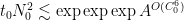
On the other hand, it is a general principle that qualitative arguments established using compactness methods ought to have quantitative analogues that replace the use of compactness by more complicated substitutes that give effective bounds; see for instance these previous blog posts for more discussion. I therefore was interested in trying to obtain a quantitative version of this blowup criterion that gave reasonably good effective bounds (in particular, my objective was to avoid truly enormous bounds such as tower-exponential or Ackermann function bounds, which often arise if one “naively” tries to make a compactness argument effective). In particular, I obtained the following triple-exponential quantitative regularity bounds:

Theorem 1 If {u} is a classical solution to Navier-Stokes on {[0,T) \times {\bf R}^3} with

\displaystyle \| u \|_{L^\infty_t L^3_x([0,T) \times {\bf R}^3)} \leq A \ \ \ \ \ (1)


for some {A \geq 2}, then

\displaystyle | \nabla^j u(t,x)| \leq \exp\exp\exp(A^{O(1)}) t^{-\frac{j+1}{2}}

and

\displaystyle | \nabla^j \omega(t,x)| \leq \exp\exp\exp(A^{O(1)}) t^{-\frac{j+2}{2}}

for {(t,x) \in [0,T) \times {\bf R}^3} and {j=0,1}.

As a corollary, one can now improve the Escauriaza-Seregin-Sverak blowup criterion to

\displaystyle \limsup_{t \rightarrow T_*} \frac{\|u(t) \|_{L^3_x({\bf R}^3)}}{(\log\log\log \frac{1}{T_*-t})^c} = +\infty

for some absolute constant {c>0}, which to my knowledge is the first (very slightly) supercritical blowup criterion for Navier-Stokes in the literature.

The proof uses many of the same quantitative inputs as previous arguments, most notably the Carleman inequalities used to establish unique continuation and backwards uniqueness theorems for backwards heat equations, but also some additional techniques that make the quantitative bounds more efficient. The proof focuses initially on points of concentration of the solution, which we define as points {(t_0,x_0)} where there is a frequency {N_0} for which one has the bound

\displaystyle |N_0^{-1} P_{N_0} u(t_0,x_0)| \geq A^{-C_0} \ \ \ \ \ (2)


for a large absolute constant {C_0}, where {P_{N_0}} is a Littlewood-Paley projection to frequencies {\sim N_0}. (This can be compared with the upper bound of {O(A)} for the quantity on the left-hand side that follows from (1).) The factor of {N_0^{-1}} normalises the left-hand side of (2) to be dimensionless (i.e., critical). The main task is to show that the dimensionless quantity {t_0 N_0^2} cannot get too large; in particular, we end up establishing a bound of the form

\displaystyle t_0 N_0^2 \lesssim \exp\exp\exp A^{O(C_0^6)}

from which the above theorem ends up following from a routine adaptation of the local well-posedness and regularity theory for Navier-Stokes.

The strategy is to show that any concentration such as (2) when {t_0 N_0^2} is large must force a significant component of the {L^3_x} norm of {u(t_0)} to also show up at many other locations than {x_0}, which eventually contradicts (1) if one can produce enough such regions of non-trivial {L^3_x} norm. (This can be viewed as a quantitative variant of the “rigidity” theorems in some of the previous proofs of the Escauriaza-Seregin-Sverak theorem that rule out solutions that exhibit too much “compactness” or “almost periodicity” in the {L^3_x} topology.) The chain of causality that leads from a concentration (2) at {(t_0,x_0)} to significant {L^3_x} norm at other regions of the time slice {t_0 \times {\bf R}^3} is somewhat involved (though simpler than the much more convoluted schemes I initially envisaged for this argument):

  1. Firstly, by using Duhamel’s formula, one can show that a concentration (2) can only occur (with {t_0 N_0^2} large) if there was also a preceding concentration

    \displaystyle |N_1^{-1} P_{N_1} u(t_1,x_1)| \geq A^{-C_0} \ \ \ \ \ (3)


    at some slightly previous point {(t_1,x_1)} in spacetime, with {N_1} also close to {N_0} (more precisely, we have {t_1 = t_0 - A^{-O(C_0^3)} N_0^{-2}}, {N_1 = A^{O(C_0^2)} N_0}, and {x_1 = x_0 + O( A^{O(C_0^4)} N_0^{-1})}). This can be viewed as a sort of contrapositive of a “local regularity theorem”, such as the ones established by Caffarelli, Kohn, and Nirenberg. A key point here is that the lower bound {A^{-C_0}} in the conclusion (3) is precisely the same as the lower bound in (2), so that this backwards propagation of concentration can be iterated.

  2. Iterating the previous step, one can find a sequence of concentration points

    \displaystyle |N_n^{-1} P_{N_n} u(t_n,x_n)| \geq A^{-C_0} \ \ \ \ \ (4)


    with the {(t_n,x_n)} propagating backwards in time; by using estimates ultimately resulting from the dissipative term in the energy identity, one can extract such a sequence in which the {t_0-t_n} increase geometrically with time, the {N_n} are comparable (up to polynomial factors in {A}) to the natural frequency scale {(t_0-t_n)^{-1/2}}, and one has {x_n = x_0 + O( |t_0-t_n|^{1/2} )}. Using the “epochs of regularity” theory that ultimately dates back to Leray, and tweaking the {t_n} slightly, one can also place the times {t_n} in intervals {I_n} (of length comparable to a small multiple of {|t_0-t_n|}) in which the solution is quite regular (in particular, {u, \nabla u, \omega, \nabla \omega} enjoy good {L^\infty_t L^\infty_x} bounds on {I_n \times {\bf R}^3}).

  3. The concentration (4) can be used to establish a lower bound for the {L^2_t L^2_x} norm of the vorticity {\omega} near {(t_n,x_n)}. As is well known, the vorticity obeys the vorticity equation

    \displaystyle \partial_t \omega = \Delta \omega - (u \cdot \nabla) \omega + (\omega \cdot \nabla) u.

    In the epoch of regularity {I_n \times {\bf R}^3}, the coefficients {u, \nabla u} of this equation obey good {L^\infty_x} bounds, allowing the machinery of Carleman estimates to come into play. Using a Carleman estimate that is used to establish unique continuation results for backwards heat equations, one can propagate this lower bound to also give lower {L^2} bounds on the vorticity (and its first derivative) in annuli of the form {\{ (t,x) \in I_n \times {\bf R}^3: R \leq |x-x_n| \leq R' \}} for various radii {R,R'}, although the lower bounds decay at a gaussian rate with {R}.

  4. Meanwhile, using an energy pigeonholing argument of Bourgain (which, in this Navier-Stokes context, is actually an enstrophy pigeonholing argument), one can locate some annuli {\{ x \in {\bf R}^3: R \leq |x-x_n| \leq R'\}} where (a slightly normalised form of) the entrosphy is small at time {t=t_n}; using a version of the localised enstrophy estimates from a previous paper of mine, one can then propagate this sort of control forward in time, obtaining an “annulus of regularity” of the form {\{ (t,x) \in [t_n,t_0] \times {\bf R}^3: R_n \leq |x-x_n| \leq R'_n\}} in which one has good estimates; in particular, one has {L^\infty_x} type bounds on {u, \nabla u, \omega, \nabla \omega} in this cylindrical annulus.
  5. By intersecting the previous epoch of regularity {I_n \times {\bf R}^3} with the above annulus of regularity, we have some lower bounds on the {L^2} norm of the vorticity (and its first derivative) in the annulus of regularity. Using a Carleman estimate first introduced by Escauriaza, Seregin, and Sverak, as well as a second application of the Carleman estimate used previously, one can then propagate this lower bound back up to time {t=t_0}, establishing a lower bound for the vorticity on the spatial annulus {\{ (t_0,x): R_n \leq |x-x_n| \leq R'_n \}}. By some basic Littlewood-Paley theory one can parlay this lower bound to a lower bound on the {L^3} norm of the velocity {u}; crucially, this lower bound is uniform in {n}.
  6. If {t_0 N_0^2} is very large (triple exponential in {A}!), one can then find enough scales {n} with disjoint {\{ (t_0,x): R_n \leq |x-x_n| \leq R'_n \}} annuli that the total lower bound on the {L^3_x} norm of {u(t_0)} provided by the above arguments is inconsistent with (1), thus establishing the claim.

The chain of causality is summarised in the following image:

scheme

It seems natural to conjecture that similar triply logarithmic improvements can be made to several of the other blowup criteria listed above, but I have not attempted to pursue this question. It seems difficult to improve the triple logarithmic factor using only the techniques here; the Bourgain pigeonholing argument inevitably costs one exponential, the Carleman inequalities cost a second, and the stacking of scales at the end to contradict the {L^3} upper bound costs the third.


Peter Denton, Stephen Parke, Xining Zhang, and I have just uploaded to the arXiv the short unpublished note “Eigenvectors from eigenvalues“. This note gives two proofs of a general eigenvector identity observed recently by Denton, Parke and Zhang in the course of some quantum mechanical calculations. The identity is as follows:

Theorem 1 Let {A} be an {n \times n} Hermitian matrix, with eigenvalues {\lambda_1(A),\dots,\lambda_n(A)}. Let {v_i} be a unit eigenvector corresponding to the eigenvalue {\lambda_i(A)}, and let {v_{i,j}} be the {j^{th}} component of {v_i}. Then

\displaystyle  |v_{i,j}|^2 \prod_{k=1; k \neq i}^n (\lambda_i(A) - \lambda_k(A)) = \prod_{k=1}^{n-1} (\lambda_i(A) - \lambda_k(M_j))

where {M_j} is the {n-1 \times n-1} Hermitian matrix formed by deleting the {j^{th}} row and column from {A}.

For instance, if we have

\displaystyle  A = \begin{pmatrix} a & X^* \\ X & M \end{pmatrix}

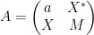
for some real number {a}, {n-1}-dimensional vector {X}, and {n-1 \times n-1} Hermitian matrix {M}, then we have

\displaystyle  |v_{i,1}|^2 = \frac{\prod_{k=1}^{n-1} (\lambda_i(A) - \lambda_k(M))}{\prod_{k=1; k \neq i}^n (\lambda_i(A) - \lambda_k(A))} \ \ \ \ \ (1)

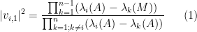
assuming that the denominator is non-zero.

Once one is aware of the identity, it is not so difficult to prove it; we give two proofs, each about half a page long, one of which is based on a variant of the Cauchy-Binet formula, and the other based on properties of the adjugate matrix. But perhaps it is surprising that such a formula exists at all; one does not normally expect to learn much information about eigenvectors purely from knowledge of eigenvalues. In the random matrix theory literature, for instance in this paper of Erdos, Schlein, and Yau, or this later paper of Van Vu and myself, a related identity has been used, namely

\displaystyle  |v_{i,1}|^2 = \frac{1}{1 + \| (M-\lambda_i(A))^{-1} X \|^2}, \ \ \ \ \ (2)

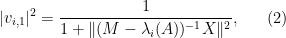
but it is not immediately obvious that one can derive the former identity from the latter. (I do so below the fold; we ended up not putting this proof in the note as it was longer than the two other proofs we found. I also give two other proofs below the fold, one from a more geometric perspective and one proceeding via Cramer’s rule.) It was certainly something of a surprise to me that there is no explicit appearance of the {a,X} components of {A} in the formula (1) (though they do indirectly appear through their effect on the eigenvalues {\lambda_k(A)}; for instance from taking traces one sees that {a = \sum_{k=1}^n \lambda_k(A) - \sum_{k=1}^{n-1} \lambda_k(M)}).

One can get some feeling of the identity (1) by considering some special cases. Suppose for instance that
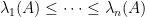
 {A} is a diagonal matrix with all distinct entries. The upper left entry {a} of {A} is one of the eigenvalues of {A}. If it is equal to {\lambda_i(A)}, then the eigenvalues of {M} are the other {n-1} eigenvalues of {A}, and now the left and right-hand sides of (1) are equal to {1}. At the other extreme, if {a} is equal to a different eigenvalue of {A}, then {\lambda_i(A)} now appears as an eigenvalue of {M}, and both sides of (1) now vanish. More generally, if we order the eigenvalues {\lambda_1(A) \leq \dots \leq \lambda_n(A)} and {\lambda_1(M) \leq \dots \leq \lambda_{n-1}(M)}, then the Cauchy interlacing inequalities tell us that

\displaystyle  0 \leq \lambda_i(A) - \lambda_k(M) \leq \lambda_i(A) - \lambda_k(A)

for {1 \leq k < i}, and

\displaystyle  \lambda_i(A) - \lambda_{k+1}(A) \leq \lambda_i(A) - \lambda_k(M) < 0

for {i \leq k \leq n-1}, so that the right-hand side of (1) lies between {0} and {1}, which is of course consistent with (1) as {v_i} is a unit vector. Thus the identity relates the coefficient sizes of an eigenvector with the extent to which the Cauchy interlacing inequalities are sharp.

Read the rest of this entry »

Archives