
You are currently browsing the tag archive for the ‘equidistribution’ tag.
Define the Collatz map 


for all 


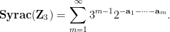
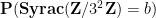
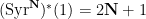
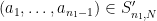
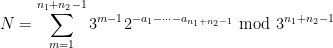
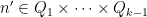
Definition 1 (Syracuse random variables) For any natural number
, a Syracuse random variable
on the cyclic group
is defined as a random variable of the form
where
are independent copies of a geometric random variable
on the natural numbers with mean
, thus
} for
. In (2) the arithmetic is performed in the ring


Thus for instance


and so forth. After reversing the labeling of the 


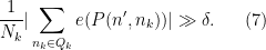
The probability density function 


when 
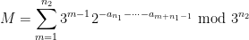
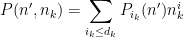
The relationship of these random variables to the Collatz problem can be explained as follows. Let 

where the 


for all
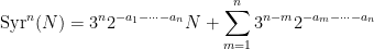
where the natural numbers 

so in particular
Heuristically, one expects the 
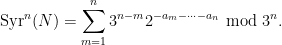
The Syracuse random variables 

Equivalently, 
for all integers 

Thus for instance 


There is also an easy submultiplicativity result:
Lemma 2 For any natural numbers
, we have

Proof: Let
If we let 


 , then
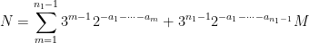
with 

for all 
so that 
for each

From this lemma we see that 


Proposition 3 Suppose that
as
). Then
as
, or equivalently


 .
.I prove this proposition below the fold. A variant of the argument shows that for any value of 

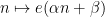
![{f: [0,1] \rightarrow [0,1]}](https://s0.wp.com/latex.php?latex=%7Bf%3A+%5B0%2C1%5D+%5Crightarrow+%5B0%2C1%5D%7D&bg=ffffff&fg=000000&s=0&c=20201002)


A sequence 

for some real numbers 


with 

These sequences arise in various “complexity one” problems in arithmetic combinatorics and ergodic theory. For instance, if 


can be shown to be an almost periodic sequence, plus an error term 

This can be established in a number of ways, for instance by writing 


In the last two decades or so, it has become clear that there are natural higher order versions of these concepts, in which linear polynomials such as 


For technical reasons (having to do with the non-trivial topological structure on nilmanifolds), it will be convenient to work with vector-valued sequences, that take values in a finite-dimensional complex vector space 


This product is associative and bilinear, and also commutative up to permutation of the indices. It also interacts well with the Hermitian norm

since we have 
The traditional definition of a basic nilsequence (as defined for instance by Bergelson, Host, and Kra) is as follows:
Definition 1 (Basic nilsequence, first definition) A nilmanifold of step at most
is a quotient
, where
is a connected, simply connected nilpotent Lie group of step at most
-fold commutators vanish) and
is a discrete cocompact lattice in
, where
,
, and
is a continuous function.
For instance, it is not difficult using this definition to show that a sequence is a basic nilsequence of degree at most 

Nowadays, and particularly when one needs to understand the “single-scale” equidistribution properties of nilsequences, it is more convenient (as is for instance done in this ICM paper of Green) to use an alternate definition of a nilsequence as follows.
Definition 2 Let
. A filtered group of degree at most
of subgroups
with
and
for
. A polynomial sequence
into a filtered group is a function such that
for all
and
, where
is the difference operator. A filtered nilmanifold of degree at most
is a quotient
are connected, simply connected nilpotent filtered Lie group, and
is a discrete cocompact subgroup of
, where
is a continuous function which is
for all
.
One can easily identify a 

It is easy to see that any sequence that is a basic nilsequence of degree at most 

where 


The other key example is a sequence of the form
where 


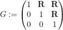
with the lower central series filtration 
![{G_2= [G,G] = \begin{pmatrix} 1 &0 & {\bf R} \\ 0 & 1 & 0 \\ 0 & 0 & 1 \end{pmatrix}}](https://s0.wp.com/latex.php?latex=%7BG_2%3D+%5BG%2CG%5D+%3D+%5Cbegin%7Bpmatrix%7D+1+%260+%26+%7B%5Cbf+R%7D+%5C%5C+0+%26+1+%26+0+%5C%5C+0+%26+0+%26+1+%5Cend%7Bpmatrix%7D%7D&bg=ffffff&fg=000000&s=0&c=20201002)


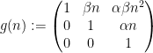
and 

one easily verifies that this function is indeed 


will be a basic nilsequence if 
A nilsequence of degree at most 


is equal to a nilsequence of degree at most 

It is easy to see that a sequence 


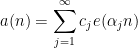
Now we turn to the notion of a nilcharacter, as defined in this paper of Ben Green, Tamar Ziegler, and myself:
Definition 3 (Nilcharacters) Let
. A sub-nilcharacter of degree
of degree at most
for all
, where
is a continuous homomorphism
. (Note from (1) and
must map
to
.) If in addition one has
for all
a nilcharacter of degree

In the degree one case 


where 

for all 


We claim that every degree 


and then

becomes a degree 
As we shall show below, nilsequences can be approximated uniformly by linear combinations of nilcharacters, in much the same way that quasiperiodic or almost periodic sequences can be approximated uniformly by linear combinations of linear phases. In particular, nilcharacters can be used as “obstructions to uniformity” in the sense of the inverse theory of the Gowers uniformity norms.
The space of degree
Definition 4 Let
,
are equivalent if
is equal (as a sequence) to a basic nilsequence of degree at most
of such a nilcharacter will be called the symbol of that nilcharacter (in analogy to the symbol of a differential or pseudodifferential operator), and the collection of such symbols will be denoted
.
As we shall see below the fold, 


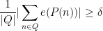
The equidistribution theorem asserts that if 


for any continuous (or equivalently, for any smooth) function 

for any non-zero integer 


One can then ask for more quantitative information about the decay of exponential sums of 


Lemma 1 (Geometric series formula, inverse form) Let
be an arithmetic progression of length at most
, and let
be a linear polynomial for some
. If
for some
, then there exists a subprogression
of
such that
varies by at most
on
of length at most

Proof: By a linear change of variable we may assume that 


and so 

Thus, in order for a linear phase 
As is well known, this phenomenon generalises to higher order polynomials. To achieve this, we need two elementary additional lemmas. The first relates the exponential sums of 
Lemma 2 (Van der Corput lemma, inverse form) Let
be an arbitrary function such that
for some
integers
, there exists a subprogression
of


Proof: Squaring (1), we see that

We write 

where 


for
The second lemma (which we recycle from this previous blog post) is a variant of the equidistribution theorem.
Lemma 3 (Vinogradov lemma) Let
be an interval for some
be such that
for at least
values of
, for some
. Then either
or
or else there is a natural number
such that


Proof: We may assume that 


We take 


If 


By hypothesis, 


We conclude that for fixed 

![{[n, n + \frac{1}{10 |\kappa|}]}](https://s0.wp.com/latex.php?latex=%7B%5Bn%2C+n+%2B+%5Cfrac%7B1%7D%7B10+%7C%5Ckappa%7C%7D%5D%7D&bg=ffffff&fg=000000&s=0&c=20201002)


and the claim follows.
Now we can quickly obtain a higher degree version of Lemma 1:
Proposition 4 (Weyl exponential sum estimate, inverse form) Let
be a polynomial of some degree at most
for some
such that
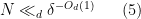
Proof: We induct on 

By rescaling we may assume ![{Q \subset [0,N] \cap {\bf Z}}](https://s0.wp.com/latex.php?latex=%7BQ+%5Csubset+%5B0%2CN%5D+%5Ccap+%7B%5Cbf+Z%7D%7D&bg=ffffff&fg=000000&s=0&c=20201002)
![{h \in [-N,N] \cap {\bf Z}}](https://s0.wp.com/latex.php?latex=%7Bh+%5Cin+%5B-N%2CN%5D+%5Ccap+%7B%5Cbf+Z%7D%7D&bg=ffffff&fg=000000&s=0&c=20201002)

for some interval ![{I_h \subset [0,N] \cap {\bf Z}}](https://s0.wp.com/latex.php?latex=%7BI_h+%5Csubset+%5B0%2CN%5D+%5Ccap+%7B%5Cbf+Z%7D%7D&bg=ffffff&fg=000000&s=0&c=20201002)


![{[-\delta^{-O(1)} N, \delta^{-O(1)} N] \cap {\bf Z}}](https://s0.wp.com/latex.php?latex=%7B%5B-%5Cdelta%5E%7B-O%281%29%7D+N%2C+%5Cdelta%5E%7B-O%281%29%7D+N%5D+%5Ccap+%7B%5Cbf+Z%7D%7D&bg=ffffff&fg=000000&s=0&c=20201002)


In the former case the claim is trivial (just take
We partition 

so by the pigeonhole principle, we have

for at least one such progression 


and hence by induction hypothesis we may find a subprogression 


This gives the following corollary (also given as Exercise 16 in this previous blog post):
Corollary 5 (Weyl exponential sum estimate, inverse form II) Let
. If
for some
such that
for all

One can obtain much better exponents here using Vinogradov’s mean value theorem; see Theorem 1.6 this paper of Wooley. (Thanks to Mariusz Mirek for this reference.) However, this weaker result already suffices for many applications, and does not need any result as deep as the mean value theorem.
Proof: To simplify notation we allow implied constants to depend on 


Applying Proposition 4, we can find a natural number 


![{I' \subset [0,N] \cap {\bf Z}}](https://s0.wp.com/latex.php?latex=%7BI%27+%5Csubset+%5B0%2CN%5D+%5Ccap+%7B%5Cbf+Z%7D%7D&bg=ffffff&fg=000000&s=0&c=20201002)


For future reference we also record a higher degree version of the Vinogradov lemma.
Lemma 6 (Polynomial Vinogradov lemma) Let
for at least
or else there is a natural number
for all


Proof: We induct on 
For each ![{h \in [-2N,2N] \cap {\bf Z}}](https://s0.wp.com/latex.php?latex=%7Bh+%5Cin+%5B-2N%2C2N%5D+%5Ccap+%7B%5Cbf+Z%7D%7D&bg=ffffff&fg=000000&s=0&c=20201002)

![{n \in [-N,N] \cap {\bf Z}}](https://s0.wp.com/latex.php?latex=%7Bn+%5Cin+%5B-N%2CN%5D+%5Ccap+%7B%5Cbf+Z%7D%7D&bg=ffffff&fg=000000&s=0&c=20201002)

![{\sum_{h \in [-2N,2N] \cap {\bf Z}} N_h \gg \delta^2 N^2}](https://s0.wp.com/latex.php?latex=%7B%5Csum_%7Bh+%5Cin+%5B-2N%2C2N%5D+%5Ccap+%7B%5Cbf+Z%7D%7D+N_h+%5Cgg+%5Cdelta%5E2+N%5E2%7D&bg=ffffff&fg=000000&s=0&c=20201002)


for 


Since 
for

We can again assume it is the latter that holds. This implies that 

for
The above results also extend to higher dimensions. Here is the higher dimensional version of Proposition 4:
Proposition 7 (Multidimensional Weyl exponential sum estimate, inverse form) Let
and
, and let
be arithmetic progressions of length at most
for each
. Let
be a polynomial of degrees at most
in each of the
separately. If
for some
of
with
for each
.
A much more general statement, in which the polynomial phase 
Proof: We induct on 


By a linear change of variables, we may assume that ![{Q_i \subset [0,N_i] \cap {\bf Z}}](https://s0.wp.com/latex.php?latex=%7BQ_i+%5Csubset+%5B0%2CN_i%5D+%5Ccap+%7B%5Cbf+Z%7D%7D&bg=ffffff&fg=000000&s=0&c=20201002)
We write 

and the claim then follows from the induction hypothesis. Thus we may assume that 

By the triangle inequality, we have
The inner sum is 

for some polynomials 


for 

for all 

where 


Applying Lemma 6 in the 


for all 

whenever 


An inspection of the proof of the above result (or alternatively, by combining the above result again with many applications of Lemma 6) reveals the following general form of Proposition 4, which was posed as Exercise 17 in this previous blog post, but had a slight misprint in it (it did not properly treat the possibility that some of the 
Proposition 8 (Multidimensional Weyl exponential sum estimate, inverse form, II) Let
be a discrete interval for some
. Let
be a polynomial in
for some
. If
for some
, or else there is a natural number
such that


 for
for Again, the factor of 


![{\sum_{n_1 \in \{0,1\}} \sum_{n_2 \in [1,N] \cap {\bf Z}} e( \alpha n_1 n_2)}](https://s0.wp.com/latex.php?latex=%7B%5Csum_%7Bn_1+%5Cin+%5C%7B0%2C1%5C%7D%7D+%5Csum_%7Bn_2+%5Cin+%5B1%2CN%5D+%5Ccap+%7B%5Cbf+Z%7D%7D+e%28+%5Calpha+n_1+n_2%29%7D&bg=ffffff&fg=000000&s=0&c=20201002)
In Notes 5, we saw that the Gowers uniformity norms on vector spaces 

Now we study the analogous situation on cyclic groups 

Traditionally, nilsequences have been defined in terms of linear orbits 

A polynomial phase 


In these notes we set out the basic theory for these nilsequences, including their equidistribution theory (which generalises the equidistribution theory of polynomial flows on tori from Notes 1) and show that they are indeed obstructions to the Gowers norm being small. This leads to the inverse conjecture for the Gowers norms that shows that the Gowers norms on cyclic groups are indeed controlled by these sequences.
In the previous lectures, we have focused mostly on the equidistribution or linear patterns on a subset of the integers ![{[N]}](https://s0.wp.com/latex.php?latex=%7B%5BN%5D%7D&bg=ffffff&fg=000000&s=0&c=20201002)


The additive combinatorics of the integers 

The starting point for this course (Notes 1) was the study of equidistribution of polynomials 


(Linear) Fourier analysis can be viewed as a tool to study an arbitrary function 


In this course we will be studying higher-order correlations, such as the correlation of 


Such sums are closely related to the distribution of expressions such as 


More generally, to find arithmetic progressions such as 


The theory of equidistribution of polynomial orbits was developed in the linear case by Dirichlet and Kronecker, and in the polynomial case by Weyl. There are two regimes of interest; the (qualitative) asymptotic regime in which the scale parameter
We will view the equidistribution theory of polynomial orbits as a special case of Ratner’s theorem, which we will study in more generality later in this course.
For the finitary portion of the course, we will be using asymptotic notation: 


Today, Prof. Margulis continued his lecture series, focusing on two specific examples of homogeneous dynamics applications to number theory, namely counting lattice points on algebraic varieties, and quantitative versions of the Oppenheim conjecture. (Due to lack of time, the third application mentioned in the previous lecture, namely metric theory of Diophantine approximation, was not covered.)
The final distinguished lecture series for the academic year here at UCLA is being given this week by Gregory Margulis, who is giving three lectures on “homogeneous dynamics and number theory”. In his first lecture, Prof. Margulis surveyed some classical problems in number theory that turn out, rather surprisingly, to have more or less equivalent counterparts in homogeneous dynamics – the theory of dynamical systems on homogeneous spaces 
As usual, any errors in this post are due to my transcription of the talk.
This week I was in Columbus, Ohio, attending a conference on equidistribution on manifolds. I talked about my recent paper with Ben Green on the quantitative behaviour of polynomial sequences in nilmanifolds, which I have blogged about previously. During my talk (and inspired by the immediately preceding talk of Vitaly Bergelson), I stated explicitly for the first time a generalisation of the van der Corput trick which morally underlies our paper, though it is somewhat buried there as we specialised it to our application at hand (and also had to deal with various quantitative issues that made the presentation more complicated). After the talk, several people asked me for a more precise statement of this trick, so I am presenting it here, and as an application reproving an old theorem of Leon Green that gives a necessary and sufficient condition as to whether a linear sequence 
UPDATE, Feb 2013: It has been pointed out to me by Pavel Zorin that this argument does not fully recover the theorem of Leon Green; to cover all cases, one needs the more complicated van der Corput argument in our paper.
Ben Green and I have just uploaded our joint paper, “The distribution of polynomials over finite fields, with applications to the Gowers norms“, to the arXiv, and submitted to Contributions to Discrete Mathematics. This paper, which we first announced at the recent FOCS meeting, and then gave an update on two weeks ago on this blog, is now in final form. It is being made available simultaneously with a closely related paper of Lovett, Meshulam, and Samorodnitsky.
In the previous post on this topic, I focused on the negative results in the paper, and in particular the fact that the inverse conjecture for the Gowers norm fails for certain degrees in low characteristic. Today, I’d like to focus instead on the positive results, which assert that for polynomials in many variables over finite fields whose degree is less than the characteristic of the field, one has a satisfactory theory for the distribution of these polynomials. Very roughly speaking, the main technical results are:
- A regularity lemma: Any polynomial can be expressed as a combination of a bounded number of other polynomials which are regular, in the sense that no non-trivial linear combination of these polynomials can be expressed efficiently in terms of lower degree polynomials.
- A counting lemma: A regular collection of polynomials behaves as if the polynomials were selected randomly. In particular, the polynomials are jointly equidistributed.

Recent Comments