
You are currently browsing the monthly archive for June 2020.
Kari Astala, Steffen Rohde, Eero Saksman and I have (finally!) uploaded to the arXiv our preprint “Homogenization of iterated singular integrals with applications to random quasiconformal maps“. This project started (and was largely completed) over a decade ago, but for various reasons it was not finalised until very recently. The motivation for this project was to study the behaviour of “random” quasiconformal maps. Recall that a (smooth) quasiconformal map is a homeomorphism 

 ; this can be viewed as a deformation of the Cauchy-Riemann equation
  . Assuming that
  is asymptotic to
  at infinity, one can (formally, at least) solve for
  in terms of
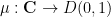
  using the Beurling transform
 if
if  is a random field that oscillates at some fine spatial scale
  . A simple model to keep in mind is
 ![\displaystyle \mu_\delta(z) = \varphi(z) \sum_{n \in {\bf Z}^2} \epsilon_n 1_{n\delta + [0,\delta]^2}(z) \ \ \ \ \ (1)](https://s0.wp.com/latex.php?latex=%5Cdisplaystyle++%5Cmu_%5Cdelta%28z%29+%3D+%5Cvarphi%28z%29+%5Csum_%7Bn+%5Cin+%7B%5Cbf+Z%7D%5E2%7D+%5Cepsilon_n+1_%7Bn%5Cdelta+%2B+%5B0%2C%5Cdelta%5D%5E2%7D%28z%29+%5C+%5C+%5C+%5C+%5C+%281%29&bg=ffffff&fg=000000&s=0&c=20201002)
 are independent random signs and
  is a bump function. For models such as these, we show that a homogenisation occurs in the limit
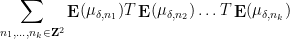
  ; each multilinear expression
 to a lacunary sequence) to a deterministic limit, and the associated quasiconformal map
  similarly converges weakly in probability (or almost surely). (Results of this latter type were also recently obtained by Ivrii and Markovic by a more geometric method which is simpler, but is applied to a narrower class of Beltrami coefficients.) In the specific case (1), the limiting quasiconformal map is just the identity map
  , but if for instance replaces the
  by non-symmetric random variables then one can have significantly more complicated limits. The convergence theorem for multilinear expressions such as is not specific to the Beurling transform
  ; any other translation and dilation invariant singular integral can be used here.
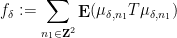
The random expression (2) is somewhat reminiscent of a moment of a random matrix, and one can start computing it analogously. For instance, if one has a decomposition 

 .
.
If all the 
 collide with each other, preventing one from easily factoring the expression. A typical problematic contribution for instance would be a sum of the form

 in the latter sum, then it splits into
 requires an inclusion-exclusion argument that creates some notational headaches but is ultimately manageable.) As the name suggests, the non-split configurations such as (4) cannot be factored in this fashion, and are the most difficult to handle. A direct computation using the triangle inequality (and a certain amount of combinatorics and induction) reveals that these sums are somewhat localised, in that dyadic portions such as
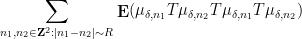
 (when measured in suitable function space norms), basically because of the large number of times one has to transition back and forth between
  and
and  . Thus, morally at least, the dominant contribution to a non-split sum such as (4) comes from the local portion when
  . From the translation and dilation invariance of this type of expression then simplifies to something like
 , and this can be shown to converge to a weak limit as .
In principle all of these limits are computable, but the combinatorics is remarkably complicated, and while there is certainly some algebraic structure to the calculations, it does not seem to be easily describable in terms of an existing framework (e.g., that of free probability).

Recent Comments