Finitary consequences of the invariant subspace problem

One of the most notorious open problems in functional analysis is the invariant subspace problem for Hilbert spaces, which I will state here as a conjecture:

Conjecture 1 (Invariant Subspace Problem, ISP0) Let be an infinite dimensional complex Hilbert space, and let be a bounded linear operator. Then contains a proper closed invariant subspace (thus ).

As stated this conjecture is quite infinitary in nature. Just for fun, I set myself the task of trying to find an equivalent reformulation of this conjecture that only involved finite-dimensional spaces and operators. This turned out to be somewhat difficult, but not entirely impossible, if one adopts a sufficiently generous version of “finitary” (cf. my discussion of how to finitise the infinitary pigeonhole principle). Unfortunately, the finitary formulation that I arrived at ended up being rather complicated (in particular, involving the concept of a “barrier”), and did not obviously suggest a path to resolving the conjecture; but it did at least provide some simpler finitary consequences of the conjecture which might be worth focusing on as subproblems.

I should point out that the arguments here are quite “soft” in nature and are not really addressing the heart of the invariant subspace problem; but I think it is still of interest to observe that this problem is not purely an infinitary problem, and does have some non-trivial finitary consequences.

I am indebted to Henry Towsner for many discussions on this topic.

Mini-polymath2 start time

In view of feedback, I have decided to start the mini-polymath2 project at 16:00 July 8 UTC, at which time I will select one of the 2010 IMO questions to solve.  The actual project will be run on the polymath blog; this blog will host the discussion threads and post-experiment analysis.

The uncertainty principle

A recurring theme in mathematics is that of duality: a mathematical object can either be described internally (or in physical space, or locally), by describing what physically consists of (or what kind of maps exist into ), or externally (or in frequency space, or globally), by describing what globally interacts or resonates with (or what kind of maps exist out of ). These two fundamentally opposed perspectives on the object are often dual to each other in various ways: performing an operation on may transform it one way in physical space, but in a dual way in frequency space, with the frequency space description often being a “inversion” of the physical space description. In several important cases, one is fortunate enough to have some sort of fundamental theorem connecting the internal and external perspectives. Here are some (closely inter-related) examples of this perspective:

1. Vector space duality A vector space over a field can be described either by the set of vectors inside , or dually by the set of linear functionals from to the field (or equivalently, the set of vectors inside the dual space ). (If one is working in the category of topological vector spaces, one would work instead with continuous linear functionals; and so forth.) A fundamental connection between the two is given by the Hahn-Banach theorem (and its relatives).
2. Vector subspace duality In a similar spirit, a subspace of can be described either by listing a basis or a spanning set, or dually by a list of linear functionals that cut out that subspace (i.e. a spanning set for the orthogonal complement . Again, the Hahn-Banach theorem provides a fundamental connection between the two perspectives.
3. Convex duality More generally, a (closed, bounded) convex body in a vector space can be described either by listing a set of (extreme) points whose convex hull is , or else by listing a set of (irreducible) linear inequalities that cut out . The fundamental connection between the two is given by the Farkas lemma.
4. Ideal-variety duality In a slightly different direction, an algebraic variety in an affine space can be viewed either “in physical space” or “internally” as a collection of points in , or else “in frequency space” or “externally” as a collection of polynomials on whose simultaneous zero locus cuts out . The fundamental connection between the two perspectives is given by the nullstellensatz, which then leads to many of the basic fundamental theorems in classical algebraic geometry.
5. Hilbert space duality An element in a Hilbert space can either be thought of in physical space as a vector in that space, or in momentum space as a covector on that space. The fundamental connection between the two is given by the Riesz representation theorem for Hilbert spaces.
6. Semantic-syntactic duality Much more generally still, a mathematical theory can either be described internally or syntactically via its axioms and theorems, or externally or semantically via its models. The fundamental connection between the two perspectives is given by the Gödel completeness theorem.
7. Intrinsic-extrinsic duality A (Riemannian) manifold can either be viewed intrinsically (using only concepts that do not require an ambient space, such as the Levi-Civita connection), or extrinsically, for instance as the level set of some defining function in an ambient space. Some important connections between the two perspectives includes the Nash embedding theorem and the theorema egregium.
8. Group duality A group can be described either via presentations (lists of generators, together with relations between them) or representations (realisations of that group in some more concrete group of transformations). A fundamental connection between the two is Cayley’s theorem. Unfortunately, in general it is difficult to build upon this connection (except in special cases, such as the abelian case), and one cannot always pass effortlessly from one perspective to the other.
9. Pontryagin group duality A (locally compact Hausdorff) abelian group can be described either by listing its elements , or by listing the characters (i.e. continuous homomorphisms from to the unit circle, or equivalently elements of ). The connection between the two is the focus of abstract harmonic analysis.
10. Pontryagin subgroup duality A subgroup of a locally compact abelian group can be described either by generators in , or generators in the orthogonal complement . One of the fundamental connections between the two is the Poisson summation formula.
11. Fourier duality A (sufficiently nice) function on a locally compact abelian group (equipped with a Haar measure ) can either be described in physical space (by its values at each element of ) or in frequency space (by the values at elements of the Pontryagin dual ). The fundamental connection between the two is the Fourier inversion formula.
12. The uncertainty principle The behaviour of a function at physical scales above (resp. below) a certain scale is almost completely controlled by the behaviour of its Fourier transform at frequency scales below (resp. above) the dual scale and vice versa, thanks to various mathematical manifestations of the uncertainty principle. (The Poisson summation formula can also be viewed as a variant of this principle, using subgroups instead of scales.)
13. Stone/Gelfand duality A (locally compact Hausdorff) topological space can be viewed in physical space (as a collection of points), or dually, via the algebra of continuous complex-valued functions on that space, or (in the case when is compact and totally disconnected) via the boolean algebra of clopen sets (or equivalently, the idempotents of ). The fundamental connection between the two is given by the Stone representation theorem or the (commutative) Gelfand-Naimark theorem.

I have discussed a fair number of these examples in previous blog posts (indeed, most of the links above are to my own blog). In this post, I would like to discuss the uncertainty principle, that describes the dual relationship between physical space and frequency space. There are various concrete formalisations of this principle, most famously the Heisenberg uncertainty principle and the Hardy uncertainty principle – but in many situations, it is the heuristic formulation of the principle that is more useful and insightful than any particular rigorous theorem that attempts to capture that principle. Unfortunately, it is a bit tricky to formulate this heuristic in a succinct way that covers all the various applications of that principle; the Heisenberg inequality is a good start, but it only captures a portion of what the principle tells us. Consider for instance the following (deliberately vague) statements, each of which can be viewed (heuristically, at least) as a manifestation of the uncertainty principle:

1. A function which is band-limited (restricted to low frequencies) is featureless and smooth at fine scales, but can be oscillatory (i.e. containing plenty of cancellation) at coarse scales. Conversely, a function which is smooth at fine scales will be almost entirely restricted to low frequencies.
2. A function which is restricted to high frequencies is oscillatory at fine scales, but is negligible at coarse scales. Conversely, a function which is oscillatory at fine scales will be almost entirely restricted to high frequencies.
3. Projecting a function to low frequencies corresponds to averaging out (or spreading out) that function at fine scales, leaving only the coarse scale behaviour.
4. Projecting a frequency to high frequencies corresponds to removing the averaged coarse scale behaviour, leaving only the fine scale oscillation.
5. The number of degrees of freedom of a function is bounded by the product of its spatial uncertainty and its frequency uncertainty (or more generally, by the volume of the phase space uncertainty). In particular, there are not enough degrees of freedom for a non-trivial function to be simulatenously localised to both very fine scales and very low frequencies.
6. To control the coarse scale (or global) averaged behaviour of a function, one essentially only needs to know the low frequency components of the function (and vice versa).
7. To control the fine scale (or local) oscillation of a function, one only needs to know the high frequency components of the function (and vice versa).
8. Localising a function to a region of physical space will cause its Fourier transform (or inverse Fourier transform) to resemble a plane wave on every dual region of frequency space.
9. Averaging a function along certain spatial directions or at certain scales will cause the Fourier transform to become localised to the dual directions and scales. The smoother the averaging, the sharper the localisation.
10. The smoother a function is, the more rapidly decreasing its Fourier transform (or inverse Fourier transform) is (and vice versa).
11. If a function is smooth or almost constant in certain directions or at certain scales, then its Fourier transform (or inverse Fourier transform) will decay away from the dual directions or beyond the dual scales.
12. If a function has a singularity spanning certain directions or certain scales, then its Fourier transform (or inverse Fourier transform) will decay slowly along the dual directions or within the dual scales.
13. Localisation operations in position approximately commute with localisation operations in frequency so long as the product of the spatial uncertainty and the frequency uncertainty is significantly larger than one.
14. In the high frequency (or large scale) limit, position and frequency asymptotically behave like a pair of classical observables, and partial differential equations asymptotically behave like classical ordinary differential equations. At lower frequencies (or finer scales), the former becomes a “quantum mechanical perturbation” of the latter, with the strength of the quantum effects increasing as one moves to increasingly lower frequencies and finer spatial scales.
15. Etc., etc.
16. Almost all of the above statements generalise to other locally compact abelian groups than or , in which the concept of a direction or scale is replaced by that of a subgroup or an approximate subgroup. (In particular, as we will see below, the Poisson summation formula can be viewed as another manifestation of the uncertainty principle.)

I think of all of the above (closely related) assertions as being instances of “the uncertainty principle”, but it seems difficult to combine them all into a single unified assertion, even at the heuristic level; they seem to be better arranged as a cloud of tightly interconnected assertions, each of which is reinforced by several of the others. The famous inequality is at the centre of this cloud, but is by no means the only aspect of it.

The uncertainty principle (as interpreted in the above broad sense) is one of the most fundamental principles in harmonic analysis (and more specifically, to the subfield of time-frequency analysis), second only to the Fourier inversion formula (and more generally, Plancherel’s theorem) in importance; understanding this principle is a key piece of intuition in the subject that one has to internalise before one can really get to grips with this subject (and also with closely related subjects, such as semi-classical analysis and microlocal analysis). Like many fundamental results in mathematics, the principle is not actually that difficult to understand, once one sees how it works; and when one needs to use it rigorously, it is usually not too difficult to improvise a suitable formalisation of the principle for the occasion. But, given how vague this principle is, it is difficult to present this principle in a traditional “theorem-proof-remark” manner. Even in the more informal format of a blog post, I was surprised by how challenging it was to describe my own understanding of this piece of mathematics in a linear fashion, despite (or perhaps because of) it being one of the most central and basic conceptual tools in my own personal mathematical toolbox. In the end, I chose to give below a cloud of interrelated discussions about this principle rather than a linear development of the theory, as this seemed to more closely align with the nature of this principle.

Organising mini-polymath2

This is a continuation of the preceding post regarding the setting up of the mini-polymath2 project.  From the discussion, it seems that it is best to start at some fixed time, either on July 8 or July 9, to ensure an orderly opening to the project and also so that I can select which of the six questions would be most suitable for such a project.

I have set up a placeholder wiki page for the project here, though right now it is necessarily quite bare.

There wasn’t much feedback on where to host the polymath project, but I am thinking of hosting the main project over on the polymath blog, in order to take advantage of the slightly better threading format there (numbered comments and nested comments in particular, although unfortunately there is no comment editing capability), and also because it would be technically easier to have multiple moderators on that blog.   When the project begins, I will also announce it in a brief post on this blog, which can then serve as the “meta” or “discussion” page for the project.

The one thing that I need to fix before the project begins is the starting time.   I do not know exactly when the Kazakhstan local IMO organising committee will release the full list of questions, but presumably they should be available by, say, noon July 8 at Kazazhstan time (GMT+4), or about 8am July 8 GMT, which would probably be the earliest feasible starting time.   Given that I am at GMT-8, the next reasonable starting time would be about eight hours later, at 4pm July 8 GMT.  Below is a poll regarding what times participants would most prefer and least prefer, spaced at 4 hour intervals:

I’ve set it so that up to three answers may be selected.  I am also open to other suggestions regarding the starting time.  I encourage everyone who is interested in participating to select some times for the poll.  Note: the times given are with respect to GMT.  A list of some representative time zones and their UTC offsets (which are more or less equivalent to GMT offsets, modulo daylight savings issues) can be found here.

With this feedback, I should be able to select a reasonable starting time.  The previous mini-polymath was active for about 48 hours (in particular, continuing to produce alternate solutions well after the first one was posted), and I would expect something similar here.  I am hoping therefore that provided there is some effort by participants to help bring people up to speed, that one could drop in even several hours after the formal start of the project and still be able to contribute.

Future mini-polymath project: 2010 IMO Q6?

About a year ago, as an experiment, I set up on this blog a “mini-polymath” project, in which readers were invited to collaboratively solve the sixth question on the 2009 International Mathematical Olympiad (aka “the grasshopper problem”).  After two or three days of somewhat chaotic activity, multiple solutions to this problem were obtained, and have been archived on this page.

In the post-mortem discussion of this experiment, it became clear that the project could have benefited from some more planning and organisation, for instance by setting up a wiki page early on to try to collect strategies, insights, partial results, etc.  Also, the project was opened without any advance warning or prior discussion, which led to an interesting but chaotic opening few hours to the project.

About a month from now, the 51st International Mathematical Olympiad will be held in Kazahkstan, with the actual problems being released on July 7 and 8.  Traditionally, the sixth problem of the Olympiad (which would thus be made public on July 8) is the hardest, and often the most interesting to solve.  So in the interest of getting another data point for the polymath process, I am thinking of setting up another mini-polymath for this question (though I of course do not know in advance what this question will be!).  But this time, I would like to try to plan things out well in advance, to see if this makes much of a difference in how the project unfolds.

So I would like to open a discussion among those readers who might be interested in such a project, regarding the logistics of such a project.  Some basic issues include:

1. Date and time. Clearly, the project cannot start any earlier than July 8.  One could either try to fix a specific time (to within an hour, say), to officially start the project, or one could open the thread in advance of the IMO organisers releasing the questions, and just let the first person to find the questions post them to the thread, and start the clock from there.  I assume one can rely on the honour code to refrain from privately trying to solve the question before any official starting time.
2. Location. In addition to this blog here, there is now also a dedicated polymath blog for these projects, which has some minor advantages over this one (e.g. numbered and threaded comments with wide margins).  It has fairly low levels of activity right now (though we are just starting to write up some modest progress from the ongoing Polymath4 “finding primes” project), but this may actually be a plus when running the project, to minimise cross-traffic.  Also, another benefit of the other blog is that the project can be co-administered by several people, and not just by myself.  This blog here admittedly has significantly higher traffic than the polymath blog at present, but I would certainly post a crosslink to the polymath blog if the project started.
3. Ground rules.  The rules for the first mini-polymath project can be found here.  Basically the spirit of the rules is that the objective is not to be the first to produce an individual solution, but instead to contribute to a collective solution by sharing one’s insights, even if they are small or end up being inconclusive.  (See also Tim Gowers’ original post regarding polymath projects.)   But perhaps some tweaking to the rules may be needed.  (For instance, we may want to have some semi-official role for moderators to organise the discussion.  Ideally I would prefer not to be the sole moderator, in part because I want to see the extent to which such projects can flourish independently of one key person.)
4. Set up.  It seems clear that we should have an official wiki page (probably a subpage from the polymath wiki) well in advance of the project actually starting (which could also be used to advertise the project beyond the usual readership of this blog).  Is there anything else which it might be useful to have in place before the project starts?
5. Contingency planning. It may happen that for one reason or another, 2010 IMO Q6 will not turn out to be that good of a polymath problem.  I suppose it may be sensible to reserve the right to switch to, say, 2010 IMO Q5, if need be.  This might be one place where I might exercise some unilateral judgement, as it may be difficult to quickly get consensus on these sorts of issues.   I don’t know if it’s worth discussing these sorts of possibilities in advance; it may simply be better to improvise when and if some course corrections need to be made.

Anyway, I hope that this project will be interesting, and am hoping to get some good suggestions as to how make it an instructive and enjoyable experience for all.

The Euler-Arnold equation

A (smooth) Riemannian manifold is a smooth manifold without boundary, equipped with a Riemannian metric , which assigns a length to every tangent vector at a point , and more generally assigns an inner product

to every pair of tangent vectors at a point . (We use Roman font for here, as we will need to use to denote group elements later in this post.) This inner product is assumed to symmetric, positive definite, and smoothly varying in , and the length is then given in terms of the inner product by the formula

In coordinates (and also using abstract index notation), the metric can be viewed as an invertible symmetric rank tensor , with

One can also view the Riemannian metric as providing a (self-adjoint) identification between the tangent bundle of the manifold and the cotangent bundle ; indeed, every tangent vector is then identified with the cotangent vector , defined by the formula

In coordinates, .

A fundamental dynamical system on the tangent bundle (or equivalently, the cotangent bundle, using the above identification) of a Riemannian manifold is that of geodesic flow. Recall that geodesics are smooth curves that minimise the length

There is some degeneracy in this definition, because one can reparameterise the curve without affecting the length. In order to fix this degeneracy (and also because the square of the speed is a more tractable quantity analytically than the speed itself), it is better if one replaces the length with the energy

Minimising the energy of a parameterised curve turns out to be the same as minimising the length, together with an additional requirement that the speed stay constant in time. Minimisers (and more generally, critical points) of the energy functional (holding the endpoints fixed) are known as geodesic flows. From a physical perspective, geodesic flow governs the motion of a particle that is subject to no external forces and thus moves freely, save for the constraint that it must always lie on the manifold .

One can also view geodesic flows as a dynamical system on the tangent bundle (with the state at any time given by the position and the velocity ) or on the cotangent bundle (with the state then given by the position and the momentum ). With the latter perspective (sometimes referred to as cogeodesic flow), geodesic flow becomes a Hamiltonian flow, with Hamiltonian given as

where is the inverse inner product to , which can be defined for instance by the formula

In coordinates, geodesic flow is given by Hamilton’s equations of motion

In terms of the velocity , we can rewrite these equations as the geodesic equation

where

are the Christoffel symbols; using the Levi-Civita connection , this can be written more succinctly as

If the manifold is an embedded submanifold of a larger Euclidean space , with the metric on being induced from the standard metric on , then the geodesic flow equation can be rewritten in the equivalent form

where is now viewed as taking values in , and is similarly viewed as a subspace of . This is intuitively obvious from the geometric interpretation of geodesics: if the curvature of a curve contains components that are transverse to the manifold rather than normal to it, then it is geometrically clear that one should be able to shorten the curve by shifting it along the indicated transverse direction. It is an instructive exercise to rigorously formulate the above intuitive argument. This fact also conforms well with one’s physical intuition of geodesic flow as the motion of a free particle constrained to be in ; the normal quantity then corresponds to the centripetal force necessary to keep the particle lying in (otherwise it would fly off along a tangent line to , as per Newton’s first law). The precise value of the normal vector can be computed via the second fundamental form as , but we will not need this formula here.

In a beautiful paper from 1966, Vladimir Arnold (who, sadly, passed away last week), observed that many basic equations in physics, including the Euler equations of motion of a rigid body, and also (by which is a priori a remarkable coincidence) the Euler equations of fluid dynamics of an inviscid incompressible fluid, can be viewed (formally, at least) as geodesic flows on a (finite or infinite dimensional) Riemannian manifold. And not just any Riemannian manifold: the manifold is a Lie group (or, to be truly pedantic, a torsor of that group), equipped with a right-invariant (or left-invariant, depending on one’s conventions) metric. In the context of rigid bodies, the Lie group is the group 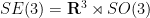of rigid motions; in the context of incompressible fluids, it is the group ) of measure-preserving diffeomorphisms. The right-invariance makes the Hamiltonian mechanics of geodesic flow in this context (where it is sometimes known as the Euler-Arnold equation or the Euler-Poisson equation) quite special; it becomes (formally, at least) completely integrable, and also indicates (in principle, at least) a way to reformulate these equations in a Lax pair formulation. And indeed, many further completely integrable equations, such as the Korteweg-de Vries equation, have since been reinterpreted as Euler-Arnold flows.

From a physical perspective, this all fits well with the interpretation of geodesic flow as the free motion of a system subject only to a physical constraint, such as rigidity or incompressibility. (I do not know, though, of a similarly intuitive explanation as to why the Korteweg de Vries equation is a geodesic flow.)

One consequence of being a completely integrable system is that one has a large number of conserved quantities. In the case of the Euler equations of motion of a rigid body, the conserved quantities are the linear and angular momentum (as observed in an external reference frame, rather than the frame of the object). In the case of the two-dimensional Euler equations, the conserved quantities are the pointwise values of the vorticity (as viewed in Lagrangian coordinates, rather than Eulerian coordinates). In higher dimensions, the conserved quantity is now the (Hodge star of) the vorticity, again viewed in Lagrangian coordinates. The vorticity itself then evolves by the vorticity equation, and is subject to vortex stretching as the diffeomorphism between the initial and final state becomes increasingly sheared.

The elegant Euler-Arnold formalism is reasonably well-known in some circles (particularly in Lagrangian and symplectic dynamics, where it can be viewed as a special case of the Euler-Poincaré formalism or Lie-Poisson formalism respectively), but not in others; I for instance was only vaguely aware of it until recently, and I think that even in fluid mechanics this perspective to the subject is not always emphasised. Given the circumstances, I thought it would therefore be appropriate to present Arnold’s original 1966 paper here. (For a more modern treatment of these topics, see the books of Arnold-Khesin and Marsden-Ratiu.)

In order to avoid technical issues, I will work formally, ignoring questions of regularity or integrability, and pretending that infinite-dimensional manifolds behave in exactly the same way as their finite-dimensional counterparts. In the finite-dimensional setting, it is not difficult to make all of the formal discussion below rigorous; but the situation in infinite dimensions is substantially more delicate. (Indeed, it is a notorious open problem whether the Euler equations for incompressible fluids even forms a global continuous flow in a reasonable topology in the first place!) However, I do not want to discuss these analytic issues here; see this paper of Ebin and Marsden for a treatment of these topics.

254B, Lecture Notes 7: The transference principle, and linear equations in primes

In this, the final lecture notes of this course, we discuss one of the motivating applications of the theory developed thus far, namely to count solutions to linear equations in primes (or in dense subsets of primes ). Unfortunately, the most famous linear equations in primes: the twin prime equation and the even Goldbach equation – remain out of reach of this technology (because the relevant affine linear forms involved are commensurate, and thus have infinite complexity with respect to the Gowers norms), but most other systems of equations, in particular that of arithmetic progressions for (or equivalently, for ) , as well as the odd Goldbach equation , are tractable.

To illustrate the main ideas, we will focus on the following result of Green:

Theorem 1 (Roth’s theorem in the primes) Let be a subset of primes whose upper density is positive. Then contains infinitely many arithmetic progressions of length three.

This should be compared with Roth’s theorem in the integers (Notes 2), which is the same statement but with the primes replaced by the integers (or natural numbers ). Indeed, Roth’s theorem for the primes is proven by transferring Roth’s theorem for the integers to the prime setting; the latter theorem is used as a “black box”. The key difficulty here in performing this transference is that the primes have zero density inside the integers; indeed, from the prime number theorem we have .

There are a number of generalisations of this transference technique. In a paper of Green and myself, we extended the above theorem to progressions of longer length (thus transferring Szemerédi’s theorem to the primes). In a series of papers (culminating in a paper to appear shortly) of Green, myself, and also Ziegler, related methods are also used to obtain an asymptotic for the number of solutions in the primes to any system of linear equations of bounded complexity. This latter result uses the full power of higher order Fourier analysis, in particular relying heavily on the inverse conjecture for the Gowers norms; in contrast, Roth’s theorem and Szemerédi’s theorem in the primes are “softer” results that do not need this conjecture.

To transfer results from the integers to the primes, there are three basic steps:

• A general transference principle, that transfers certain types of additive combinatorial results from dense subsets of the integers to dense subsets of a suitably “pseudorandom set” of integers (or more precisely, to the integers weighted by a suitably “pseudorandom measure”);
• An application of sieve theory to show that the primes (or more precisely, an affine modification of the primes) lie inside a suitably pseudorandom set of integers (or more precisely, have significant mass with respect to a suitably pseudorandom measure).
• If one is seeking asymptotics for patterns in the primes, and not simply lower bounds, one also needs to control correlations between the primes (or proxies for the primes, such as the Möbius function) with various objects that arise from higher order Fourier analysis, such as nilsequences.

The former step can be accomplished in a number of ways. For progressions of length three (and more generally, for controlling linear patterns of complexity at most one), transference can be accomplished by Fourier-analytic methods. For more complicated patterns, one can use techniques inspired by ergodic theory; more recently, simplified and more efficient methods based on duality (the Hahn-Banach theorem) have also been used. No number theory is used in this step. (In the case of transference to genuinely random sets, rather than pseudorandom sets, similar ideas appeared earlier in the graph theory setting, see this paper of Kohayakawa, Luczak, and Rodl.

The second step is accomplished by fairly standard sieve theory methods (e.g. the Selberg sieve, or the slight variants of this sieve used by Goldston and Yildirim). Remarkably, very little of the formidable apparatus of modern analytic number theory is needed for this step; for instance, the only fact about the Riemann zeta function that is truly needed is that it has a simple pole at , and no knowledge of L-functions is needed.

The third step does draw more significantly on analytic number theory techniques and results (most notably, the method of Vinogradov to compute oscillatory sums over the primes, and also the Siegel-Walfisz theorem that gives a good error term on the prime number theorem in arithemtic progressions). As these techniques are somewhat orthogonal to the main topic of this course, we shall only touch briefly on this aspect of the transference strategy.

An inverse theorem for the Gowers norm U^{s+1}[N] (announcement)

Ben Green, Tamar Ziegler, and I have just uploaded to the arXiv the note “An inverse theorem for the Gowers norm (announcement)“, not intended for publication. This is an announcement of our forthcoming solution of the inverse conjecture for the Gowers norm, which roughly speaking asserts that norm of a bounded function is large if and only if that function correlates with an -step nilsequence of bounded complexity.

The full argument is quite lengthy (our most recent draft is about 90 pages long), but this is in large part due to the presence of various technical details which are necessary in order to make the argument fully rigorous. In this 20-page announcement, we instead sketch a heuristic proof of the conjecture, relying in a number of “cheats” to avoid the above-mentioned technical details. In particular:

• In the announcement, we rely on somewhat vaguely defined terms such as “bounded complexity” or “linearly independent with respect to bounded linear combinations” or “equivalent modulo lower step errors” without specifying them rigorously. In the full paper we will use the machinery of nonstandard analysis to rigorously and precisely define these concepts.
• In the announcement, we deal with the traditional linear nilsequences rather than the polynomial nilsequences that turn out to be better suited for finitary equidistribution theory, but require more notation and machinery in order to use.
• In a similar vein, we restrict attention to scalar-valued nilsequences in the announcement, though due to topological obstructions arising from the twisted nature of the torus bundles used to build nilmanifolds, we will have to deal instead with vector-valued nilsequences in the main paper.
• In the announcement, we pretend that nilsequences can be described by bracket polynomial phases, at least for the sake of making examples, although strictly speaking bracket polynomial phases only give examples of piecewise Lipschitz nilsequences rather than genuinely Lipschitz nilsequences.

With these cheats, it becomes possible to shorten the length of the argument substantially. Also, it becomes clearer that the main task is a cohomological one; in order to inductively deduce the inverse conjecture for a given step from the conjecture for the preceding step , the basic problem is to show that a certain (quasi-)cocycle is necessarily a (quasi-)coboundary. This in turn requires a detailed analysis of the top order and second-to-top order terms in the cocycle, which requires a certain amount of nilsequence equidistribution theory and additive combinatorics, as well as a “sunflower decomposition” to arrange the various nilsequences one encounters into a usable “normal form”.

It is often the case in modern mathematics that the informal heuristic way to explain an argument looks quite different (and is significantly shorter) than the way one would formally present the argument with all the details. This seems to be particularly true in this case; at a superficial level, the full paper has a very different set of notation than the announcement, and a lot of space is invested in setting up additional machinery that one can quickly gloss over in the announcement. We hope though that the announcement can provide a “road map” to help navigate the much longer paper to come.