You are currently browsing the category archive for the ‘math.RA’ category.

Let {M_{n \times m}({\bf Z})} denote the space of {n \times m} matrices with integer entries, and let {GL_n({\bf Z})} be the group of invertible {n \times n} matrices with integer entries. The Smith normal form takes an arbitrary matrix {A \in M_{n \times m}({\bf Z})} and factorises it as {A = UDV}, where {U \in GL_n({\bf Z})}, {V \in GL_m({\bf Z})}, and {D} is a rectangular diagonal matrix, by which we mean that the principal {\min(n,m) \times \min(n,m)} minor is diagonal, with all other entries zero. Furthermore the diagonal entries of {D} are {\alpha_1,\dots,\alpha_k,0,\dots,0} for some {0 \leq k \leq \min(n,m)} (which is also the rank of {A}) with the numbers {\alpha_1,\dots,\alpha_k} (known as the invariant factors) principal divisors with {\alpha_1 | \dots | \alpha_k}. The invariant factors are uniquely determined; but there can be some freedom to modify the invertible matrices {U,V}. The Smith normal form can be computed easily; for instance, in SAGE, it can be computed calling the {{\tt smith\_form()}} function from the matrix class. The Smith normal form is also available for other principal ideal domains than the integers, but we will only be focused on the integer case here. For the purposes of this post, we will view the Smith normal form as a primitive operation on matrices that can be invoked as a “black box”.

In this post I would like to record how to use the Smith normal form to computationally manipulate two closely related classes of objects:

  • Subgroups {\Gamma \leq {\bf Z}^d} of a standard lattice {{\bf Z}^d} (or lattice subgroups for short);
  • Closed subgroups {H \leq ({\bf R}/{\bf Z})^d} of a standard torus {({\bf R}/{\bf Z})^d} (or closed torus subgroups for short).
(This arose for me due to the need to actually perform (with a collaborator) some numerical calculations with a number of lattice subgroups and closed torus subgroups.) It’s possible that all of these operations are already encoded in some existing object classes in a computational algebra package; I would be interested to know of such packages and classes for lattice subgroups or closed torus subgroups in the comments.

The above two classes of objects are isomorphic to each other by Pontryagin duality: if {\Gamma \leq {\bf Z}^d} is a lattice subgroup, then the orthogonal complement

\displaystyle  \Gamma^\perp := \{ x \in ({\bf R}/{\bf Z})^d: \langle x, \xi \rangle = 0 \forall \xi \in \Gamma \}

is a closed torus subgroup (with {\langle,\rangle: ({\bf R}/{\bf Z})^d \times {\bf Z}^d \rightarrow {\bf R}/{\bf Z}} the usual Fourier pairing); conversely, if {H \leq ({\bf R}/{\bf Z})^d} is a closed torus subgroup, then

\displaystyle  H^\perp := \{ \xi \in {\bf Z}^d: \langle x, \xi \rangle = 0 \forall x \in H \}

is a lattice subgroup. These two operations invert each other: {(\Gamma^\perp)^\perp = \Gamma} and {(H^\perp)^\perp = H}.

Example 1 The orthogonal complement of the lattice subgroup

\displaystyle  2{\bf Z} \times \{0\} = \{ (2n,0): n \in {\bf Z}\} \leq {\bf Z}^2

is the closed torus subgroup

\displaystyle  (\frac{1}{2}{\bf Z}/{\bf Z}) \times ({\bf R}/{\bf Z}) = \{ (x,y) \in ({\bf R}/{\bf Z})^2: 2x=0\} \leq ({\bf R}/{\bf Z})^2

and conversely.

Let us focus first on lattice subgroups {\Gamma \leq {\bf Z}^d}. As all such subgroups are finitely generated abelian groups, one way to describe a lattice subgroup is to specify a set {v_1,\dots,v_n \in \Gamma} of generators of {\Gamma}. Equivalently, we have

\displaystyle  \Gamma = A {\bf Z}^n

where {A \in M_{d \times n}({\bf Z})} is the matrix whose columns are {v_1,\dots,v_n}. Applying the Smith normal form {A = UDV}, we conclude that

\displaystyle  \Gamma = UDV{\bf Z}^n = UD{\bf Z}^n

so in particular {\Gamma} is isomorphic (with respect to the automorphism group {GL_d({\bf Z})} of {{\bf Z}^d}) to {D{\bf Z}^n}. In particular, we see that {\Gamma} is a free abelian group of rank {k}, where {k} is the rank of {D} (or {A}). This representation also allows one to trim the representation {A {\bf Z}^n} down to {U D'{\bf Z}^k}, where {D' \in M_{d \times k}} is the matrix formed from the {k} left columns of {D}; the columns of {UD'} then give a basis for {\Gamma}. Let us call this a trimmed representation of {A{\bf Z}^n}.

Example 2 Let {\Gamma \leq {\bf Z}^3} be the lattice subgroup generated by {(1,3,1)}, {(2,-2,2)}, {(3,1,3)}, thus {\Gamma = A {\bf Z}^3} with {A = \begin{pmatrix} 1 & 2 & 3 \\ 3 & -2 & 1 \\ 1 & 2 & 3 \end{pmatrix}}. A Smith normal form for {A} is given by

\displaystyle  A = \begin{pmatrix} 3 & 1 & 1 \\ 1 & 0 & 0 \\ 3 & 1 & 0 \end{pmatrix} \begin{pmatrix} 1 & 0 & 0 \\ 0 & 8 & 0 \\ 0 & 0 & 0 \end{pmatrix} \begin{pmatrix} 3 & -2 & 1 \\ -1 & 1 & 0 \\ 1 & 0 & 0 \end{pmatrix}

so {A{\bf Z}^3} is a rank two lattice with a basis of {(3,1,3) \times 1 = (3,1,3)} and {(1,0,1) \times 8 = (8,0,8)} (and the invariant factors are {1} and {8}). The trimmed representation is

\displaystyle  A {\bf Z}^3 = \begin{pmatrix} 3 & 1 & 1 \\ 1 & 0 & 0 \\ 3 & 1 & 0 \end{pmatrix} \begin{pmatrix} 1 & 0 \\ 0 & 8 \\ 0 & 0 \end{pmatrix} {\bf Z}^2 = \begin{pmatrix} 3 & 8 \\ 1 & 0 \\ 3 & 8 \end{pmatrix} {\bf Z}^2.

There are other Smith normal forms for {A}, giving slightly different representations here, but the rank and invariant factors will always be the same.

By the above discussion we can represent a lattice subgroup {\Gamma \leq {\bf Z}^d} by a matrix {A \in M_{d \times n}({\bf Z})} for some {n}; this representation is not unique, but we will address this issue shortly. For now, we focus on the question of how to use such data representations of subgroups to perform basic operations on lattice subgroups. There are some operations that are very easy to perform using this data representation:

  • (Applying a linear transformation) if {T \in M_{d' \times d}({\bf Z})}, so that {T} is also a linear transformation from {{\bf Z}^d} to {{\bf Z}^{d'}}, then {T} maps lattice subgroups to lattice subgroups, and clearly maps the lattice subgroup {A{\bf Z}^n} to {(TA){\bf Z}^n} for any {A \in M_{d \times n}({\bf Z})}.
  • (Sum) Given two lattice subgroups {A_1 {\bf Z}^{n_1}, A_2 {\bf Z}^{n_2} \leq {\bf Z}^d} for some {A_1 \in M_{d \times n_1}({\bf Z})}, {A_2 \in M_{d \times n_2}({\bf Z})}, the sum {A_1 {\bf Z}^{n_1} + A_2 {\bf Z}^{n_2}} is equal to the lattice subgroup {A {\bf Z}^{n_1+n_2}}, where {A = (A_1 A_2) \in M_{d \times n_1 + n_2}({\bf Z})} is the matrix formed by concatenating the columns of {A_1} with the columns of {A_2}.
  • (Direct sum) Given two lattice subgroups {A_1 {\bf Z}^{n_1} \leq {\bf Z}^{d_1}}, {A_2 {\bf Z}^{n_2} \leq {\bf Z}^{d_2}}, the direct sum {A_1 {\bf Z}^{n_1} \times A_2 {\bf Z}^{n_2}} is equal to the lattice subgroup {A {\bf Z}^{n_1+n_2}}, where {A = \begin{pmatrix} A_1 & 0 \\ 0 & A_2 \end{pmatrix} \in M_{d_1+d_2 \times n_1 + n_2}({\bf Z})} is the block matrix formed by taking the direct sum of {A_1} and {A_2}.

One can also use Smith normal form to detect when one lattice subgroup {B {\bf Z}^m \leq {\bf Z}^d} is a subgroup of another lattice subgroup {A {\bf Z}^n \leq {\bf Z}^d}. Using Smith normal form factorization {A = U D V}, with invariant factors {\alpha_1|\dots|\alpha_k}, the relation {B {\bf Z}^m \leq A {\bf Z}^n} is equivalent after some manipulation to

\displaystyle  U^{-1} B {\bf Z}^m \leq D {\bf Z}^n.

The group {U^{-1} B {\bf Z}^m} is generated by the columns of {U^{-1} B}, so this gives a test to determine whether {B {\bf Z}^{m} \leq A {\bf Z}^{n}}: the {i^{th}} row of {U^{-1} B} must be divisible by {\alpha_i} for {i=1,\dots,k}, and all other rows must vanish.

Example 3 To test whether the lattice subgroup {\Gamma'} generated by {(1,1,1)} and {(0,2,0)} is contained in the lattice subgroup {\Gamma = A{\bf Z}^3} from Example 2, we write {\Gamma'} as {B {\bf Z}^2} with {B = \begin{pmatrix} 1 & 0 \\ 1 & 2 \\ 1 & 0\end{pmatrix}}, and observe that

\displaystyle  U^{-1} B = \begin{pmatrix} 1 & 2 \\ -2 & -6 \\ 0 & 0 \end{pmatrix}.

The first row is of course divisible by {1}, and the last row vanishes as required, but the second row is not divisible by {8}, so {\Gamma'} is not contained in {\Gamma} (but {4\Gamma'} is); also a similar computation verifies that {\Gamma} is conversely contained in {\Gamma'}.

One can now test whether {B{\bf Z}^m = A{\bf Z}^n} by testing whether {B{\bf Z}^m \leq A{\bf Z}^n} and {A{\bf Z}^n \leq B{\bf Z}^m} simultaneously hold (there may be more efficient ways to do this, but this is already computationally manageable in many applications). This in principle addresses the issue of non-uniqueness of representation of a subgroup {\Gamma} in the form {A{\bf Z}^n}.

Next, we consider the question of representing the intersection {A{\bf Z}^n \cap B{\bf Z}^m} of two subgroups {A{\bf Z}^n, B{\bf Z}^m \leq {\bf Z}^d} in the form {C{\bf Z}^p} for some {p} and {C \in M_{d \times p}({\bf Z})}. We can write

\displaystyle  A{\bf Z}^n \cap B{\bf Z}^m = \{ Ax: Ax = By \hbox{ for some } x \in {\bf Z}^n, y \in {\bf Z}^m \}

\displaystyle  = (A 0) \{ z \in {\bf Z}^{n+m}: (A B) z = 0 \}

where {(A B) \in M_{d \times n+m}({\bf Z})} is the matrix formed by concatenating {A} and {B}, and similarly for {(A 0) \in M_{d \times n+m}({\bf Z})} (here we use the change of variable {z = \begin{pmatrix} x \\ -y \end{pmatrix}}). We apply the Smith normal form to {(A B)} to write

\displaystyle  (A B) = U D V

where {U \in GL_d({\bf Z})}, {D \in M_{d \times n+m}({\bf Z})}, {V \in GL_{n+m}({\bf Z})} with {D} of rank {k}. We can then write

\displaystyle  \{ z \in {\bf Z}^{n+m}: (A B) z = 0 \} = V^{-1} \{ w \in {\bf Z}^{n+m}: Dw = 0 \}

\displaystyle  = V^{-1} (\{0\}^k \times {\bf Z}^{n+m-k})

(making the change of variables {w = Vz}). Thus we can write {A{\bf Z}^n \cap B{\bf Z}^m = C {\bf Z}^{n+m-k}} where {C \in M_{d \times n+m-k}({\bf Z})} consists of the right {n+m-k} columns of {(A 0) V^{-1} \in M_{d \times n+m}({\bf Z})}.

Example 4 With the lattice {A{\bf Z}^3} from Example 2, we shall compute the intersection of {A{\bf Z}^3} with the subgroup {{\bf Z}^2 \times \{0\}}, which one can also write as {B{\bf Z}^2} with {B = \begin{pmatrix} 1 & 0 \\ 0 & 1 \\ 0 & 0 \end{pmatrix}}. We obtain a Smith normal form

\displaystyle  (A B) = \begin{pmatrix} 0 & 1 & 0 \\ 1 & 0 & 0 \\ 0 & 0 & 1 \end{pmatrix} \begin{pmatrix} 1 & 0 & 0 & 0 & 0 \\ 0 & 1 & 0 & 0 & 0 \\ 0 & 0 & 1 & 0 & 0 \end{pmatrix} \begin{pmatrix} 3 & -2 & 1 & 0 & 1 \\ 1 & 2 & 3 & 1 & 0 \\ 1 & 2 & 3 & 0 & 0 \\ 1 & 0 & 0 & 0 & 0 \\ 0 & 1 & 1 & 0 & 0 \end{pmatrix}

so {k=3}. We have

\displaystyle  (A 0) V^{-1} = \begin{pmatrix} 0 & 0 & 1 & 0 & 0 \\ 0 & 0 & 3 & 0 & -8 \\ 0 & 0 & 1 & 0 & 0 \end{pmatrix}

and so we can write {A{\bf Z}^3 \cap B{\bf Z}^2 = C{\bf Z}^2} where

\displaystyle  C = \begin{pmatrix} 0 & 0 \\ 0 & -8 \\ 0 & 0 \end{pmatrix}.

One can trim this representation if desired, for instance by deleting the first column of {C} (and replacing {{\bf Z}^2} with {{\bf Z}}). Thus the intersection of {A{\bf Z}^3} with {{\bf Z}^2 \times \{0\}} is the rank one subgroup generated by {(0,-8,0)}.

A similar calculation allows one to represent the pullback {T^{-1} (A {\bf Z}^n) \leq {\bf Z}^{d'}} of a subgroup {A{\bf Z}^n \leq {\bf Z}^d} via a linear transformation {T \in M_{d \times d'}({\bf Z})}, since

\displaystyle T^{-1} (A {\bf Z}^n) = \{ x \in {\bf Z}^{d'}: Tx = Ay \hbox{ for some } y \in {\bf Z}^m \}

\displaystyle  = (I 0) \{ z \in {\bf Z}^{d'+m}: (T A) z = 0 \}

where {(I 0) \in M_{d' \times d'+m}({\bf Z})} is the concatenation of the {d' \times d'} identity matrix {I} and the {d' \times m} zero matrix. Applying the Smith normal form to write {(T A) = UDV} with {D} of rank {k}, the same argument as before allows us to write {T^{-1}(A{\bf Z}^n) = C {\bf Z}^{d'+m-k}} where {C \in M_{d' \times d'+m-k}} consists of the right {d'+m-k} columns of {(I 0) V^{-1} \in M_{d' \times d'+m}({\bf Z})}.

Among other things, this allows one to describe lattices given by systems of linear equations and congruences in the {A{\bf Z}^n} format. Indeed, the set of lattice vectors {x \in {\bf Z}^d} that solve the system of congruences

\displaystyle  \alpha_i | x \cdot v_i \ \ \ \ \ (1)

for {i=1,\dots,k}, some natural numbers {\alpha_i}, and some lattice vectors {v_i \in {\bf Z}^d}, together with an additional system of equations

\displaystyle  x \cdot w_j = 0 \ \ \ \ \ (2)

for {j=1,\dots,l} and some lattice vectors {w_j \in {\bf Z}^d}, can be written as {T^{-1}(A {\bf Z}^k)} where {T \in M_{k+l \times d}({\bf Z})} is the matrix with rows {v_1,\dots,v_k,w_1,\dots,w_l}, and {A \in M_{k+l \times k}({\bf Z})} is the diagonal matrix with diagonal entries {\alpha_1,\dots,\alpha_k}. Conversely, any subgroup {A{\bf Z}^n} can be described in this form by first using the trimmed representation {A{\bf Z}^n = UD'{\bf Z}^k}, at which point membership of a lattice vector {x \in {\bf Z}^d} in {A{\bf Z}^n} is seen to be equivalent to the congruences

\displaystyle  \alpha_i | U^{-1} x \cdot e_i

for {i=1,\dots,k} (where {k} is the rank, {\alpha_1,\dots,\alpha_k} are the invariant factors, and {e_1,\dots,e_d} is the standard basis of {{\bf Z}^d}) together with the equations

\displaystyle  U^{-1} x \cdot e_j = 0

for {j=k+1,\dots,d}. Thus one can obtain a representation in the form (1), (2) with {l=d-k}, and {v_1,\dots,v_k,w_1,\dots,w_{d-k}} to be the rows of {U^{-1}} in order.

Example 5 With the lattice subgroup {A{\bf Z}^3} from Example 2, we have {U^{-1} = \begin{pmatrix} 0 & 1 & 0 \\ 0 & -3 & 1 \\ 1 & 0 & -1 \end{pmatrix}}, and so {A{\bf Z}^3} consists of those triples {(x_1,x_2,x_3)} which obey the (redundant) congruence

\displaystyle  1 | x_2,

the congruence

\displaystyle  8 | -3x_2 + x_3

and the identity

\displaystyle  x_1 - x_3 = 0.

Conversely, one can use the above procedure to convert the above system of congruences and identities back into a form {A' {\bf Z}^{n'}} (though depending on which Smith normal form one chooses, the end result may be a different representation of the same lattice group {A{\bf Z}^3}).

Now we apply Pontryagin duality. We claim the identity

\displaystyle  (A{\bf Z}^n)^\perp = \{ x \in ({\bf R}/{\bf Z})^d: A^Tx = 0 \}

for any {A \in M_{d \times n}({\bf Z})} (where {A^T \in M_{n \times d}({\bf Z})} induces a homomorphism from {({\bf R}/{\bf Z})^d} to {({\bf R}/{\bf Z})^n} in the obvious fashion). This can be verified by direct computation when {A} is a (rectangular) diagonal matrix, and the general case then easily follows from a Smith normal form computation (one can presumably also derive it from the category-theoretic properties of Pontryagin duality, although I will not do so here). So closed torus subgroups that are defined by a system of linear equations (over {{\bf R}/{\bf Z}}, with integer coefficients) are represented in the form {(A{\bf Z}^n)^\perp} of an orthogonal complement of a lattice subgroup. Using the trimmed form {A{\bf Z}^n = U D' {\bf Z}^k}, we see that

\displaystyle  (A{\bf Z}^n)^\perp = \{ x \in ({\bf R}/{\bf Z})^d: (UD')^T x = 0 \}

\displaystyle  = (U^{-1})^T \{ y \in ({\bf R}/{\bf Z})^d: (D')^T x = 0 \}

\displaystyle  = (U^{-1})^T (\frac{1}{\alpha_1} {\bf Z}/{\bf Z} \times \dots \times \frac{1}{\alpha_k} {\bf Z}/{\bf Z} \times ({\bf R}/{\bf Z})^{d-k}),

giving an explicit representation “in coordinates” of such a closed torus subgroup. In particular we can read off the isomorphism class of a closed torus subgroup as the product of a finite number of cyclic groups and a torus:

\displaystyle (A{\bf Z}^n)^\perp \equiv ({\bf Z}/\alpha_1 {\bf Z}) \times \dots \times ({\bf Z}/\alpha_k{\bf Z}) \times ({\bf R}/{\bf Z})^{d-k}.

Example 6 The orthogonal complement of the lattice subgroup {A{\bf Z}^3} from Example 2 is the closed torus subgroup

\displaystyle  (A{\bf Z}^3)^\perp = \{ (x_1,x_2,x_3) \in ({\bf R}/{\bf Z})^3: x_1 + 3x_2 + x_3

\displaystyle  = 2x_1 - 2x_2 + 2x_3 = 3x_1 + x_2 + 3x_3 = 0 \};

using the trimmed representation of {(A{\bf Z}^3)^\perp}, one can simplify this a little to

\displaystyle  (A{\bf Z}^3)^\perp = \{ (x_1,x_2,x_3) \in ({\bf R}/{\bf Z})^3: 3x_1 + x_2 + 3x_3

\displaystyle  = 8 x_1 + 8x_3 = 0 \}

and one can also write this as the image of the group {\{ 0\} \times (\frac{1}{8}{\bf Z}/{\bf Z}) \times ({\bf R}/{\bf Z})} under the torus isomorphism

\displaystyle  (y_1,y_2,y_3) \mapsto (y_3, y_1 - 3y_2, y_2 - y_3).

In other words, one can write

\displaystyle  (A{\bf Z}^3)^\perp = \{ (y,0,-y) + (0,-\frac{3a}{8},\frac{a}{8}): y \in {\bf R}/{\bf Z}; a \in {\bf Z}/8{\bf Z} \}

so that {(A{\bf Z}^3)^\perp} is isomorphic to {{\bf R}/{\bf Z} \times {\bf Z}/8{\bf Z}}.

We can now dualize all of the previous computable operations on subgroups of {{\bf Z}^d} to produce computable operations on closed subgroups of {({\bf R}/{\bf Z})^d}. For instance:

  • To form the intersection or sum of two closed torus subgroups {(A_1 {\bf Z}^{n_1})^\perp, (A_2 {\bf Z}^{n_2})^\perp \leq ({\bf R}/{\bf Z})^d}, use the identities

    \displaystyle  (A_1 {\bf Z}^{n_1})^\perp \cap (A_2 {\bf Z}^{n_2})^\perp = (A_1 {\bf Z}^{n_1} + A_2 {\bf Z}^{n_2})^\perp

    and

    \displaystyle  (A_1 {\bf Z}^{n_1})^\perp + (A_2 {\bf Z}^{n_2})^\perp = (A_1 {\bf Z}^{n_1} \cap A_2 {\bf Z}^{n_2})^\perp

    and then calculate the sum or intersection of the lattice subgroups {A_1 {\bf Z}^{n_1}, A_2 {\bf Z}^{n_2}} by the previous methods. Similarly, the operation of direct sum of two closed torus subgroups dualises to the operation of direct sum of two lattice subgroups.
  • To determine whether one closed torus subgroup {(A_1 {\bf Z}^{n_1})^\perp \leq ({\bf R}/{\bf Z})^d} is contained in (or equal to) another closed torus subgroup {(A_2 {\bf Z}^{n_2})^\perp \leq ({\bf R}/{\bf Z})^d}, simply use the preceding methods to check whether the lattice subgroup {A_2 {\bf Z}^{n_2}} is contained in (or equal to) the lattice subgroup {A_1 {\bf Z}^{n_1}}.
  • To compute the pull back {T^{-1}( (A{\bf Z}^n)^\perp )} of a closed torus subgroup {(A{\bf Z}^n)^\perp \leq ({\bf R}/{\bf Z})^d} via a linear transformation {T \in M_{d' \times d}({\bf Z})}, use the identity

    \displaystyle T^{-1}( (A{\bf Z}^n)^\perp ) = (T^T A {\bf Z}^n)^\perp.

    Similarly, to compute the image {T( (B {\bf Z}^m)^\perp )} of a closed torus subgroup {(B {\bf Z}^m)^\perp \leq ({\bf R}/{\bf Z})^{d'}}, use the identity

    \displaystyle T( (B{\bf Z}^m)^\perp ) = ((T^T)^{-1} B {\bf Z}^m)^\perp.

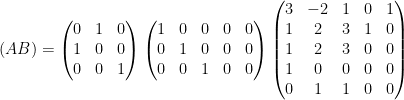
Example 7 Suppose one wants to compute the sum of the closed torus subgroup {(A{\bf Z}^3)^\perp} from Example 6 with the closed torus subgroup {\{0\}^2 \times {\bf R}/{\bf Z}}. This latter group is the orthogonal complement of the lattice subgroup {{\bf Z}^2 \times \{0\}} considered in Example 4. Thus we have {(A{\bf Z}^3)^\perp + (\{0\}^2 \times {\bf R}/{\bf Z}) = (C{\bf Z}^2)^\perp} where {C} is the matrix from Example 6; discarding the zero column, we thus have

\displaystyle (A{\bf Z}^3)^\perp + (\{0\}^2 \times {\bf R}/{\bf Z}) = \{ (x_1,x_2,x_3): -8x_2 = 0 \}.

As I have mentioned in some recent posts, I am interested in exploring unconventional modalities for presenting mathematics, for instance using media with high production value. One such recent example of this I saw was a presentation of the fundamental zero product property (or domain property) of the real numbers – namely, that ab=0 implies a=0 or b=0 for real numbers a,b – expressed through the medium of German-language rap:

EDIT: and here is a lesson on fractions, expressed through the medium of a burger chain advertisement:

I’d be interested to know what further examples of this type are out there.

SECOND EDIT: The following two examples from Wired magazine are slightly more conventional in nature, but still worth mentioning, I think. Firstly, my colleague at UCLA, Amit Sahai, presents the concept of zero knowledge proofs at various levels of technicality:

Secondly, Moon Duchin answers math questions of all sorts from Twitter:

A popular way to visualise relationships between some finite number of sets is via Venn diagrams, or more generally Euler diagrams. In these diagrams, a set is depicted as a two-dimensional shape such as a disk or a rectangle, and the various Boolean relationships between these sets (e.g., that one set is contained in another, or that the intersection of two of the sets is equal to a third) is represented by the Boolean algebra of these shapes; Venn diagrams correspond to the case where the sets are in “general position” in the sense that all non-trivial Boolean combinations of the sets are non-empty. For instance to depict the general situation of two sets {A,B} together with their intersection {A \cap B} and {A \cup B} one might use a Venn diagram such as

venn

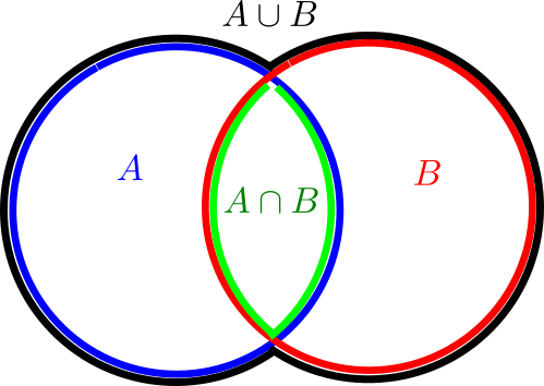
(where we have given each region depicted a different color, and moved the edges of each region a little away from each other in order to make them all visible separately), but if one wanted to instead depict a situation in which the intersection {A \cap B} was empty, one could use an Euler diagram such as

euler

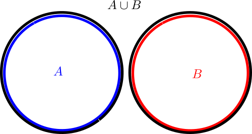
One can use the area of various regions in a Venn or Euler diagram as a heuristic proxy for the cardinality {|A|} (or measure {\mu(A)}) of the set {A} corresponding to such a region. For instance, the above Venn diagram can be used to intuitively justify the inclusion-exclusion formula

\displaystyle  |A \cup B| = |A| + |B| - |A \cap B|

for finite sets {A,B}, while the above Euler diagram similarly justifies the special case
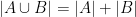
\displaystyle  |A \cup B| = |A| + |B|

for finite disjoint sets {A,B}.

While Venn and Euler diagrams are traditionally two-dimensional in nature, there is nothing preventing one from using one-dimensional diagrams such as

venn1d

or even three-dimensional diagrams such as this one from Wikipedia:

venn-3d

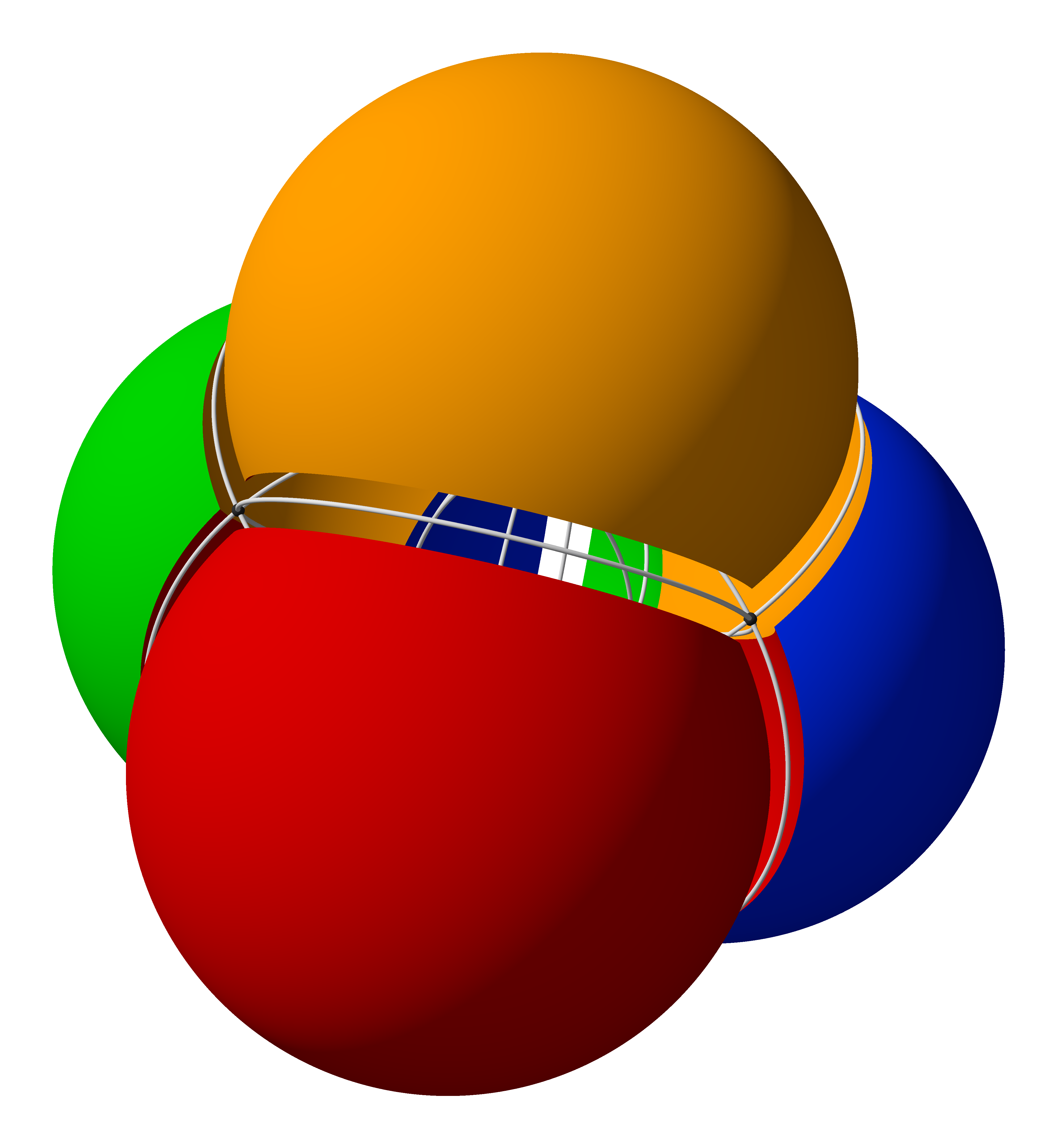
Of course, in such cases one would use length or volume as a heuristic proxy for cardinality or measure, rather than area.

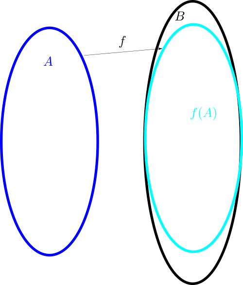
With the addition of arrows, Venn and Euler diagrams can also accommodate (to some extent) functions between sets. Here for instance is a depiction of a function {f: A \rightarrow B}, the image {f(A)} of that function, and the image {f(A')} of some subset {A'} of {A}:

afb

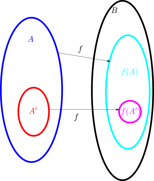
Here one can illustrate surjectivity of {f: A \rightarrow B} by having {f(A)} fill out all of {B}; one can similarly illustrate injectivity of {f} by giving {f(A)} exactly the same shape (or at least the same area) as {A}. So here for instance might be how one would illustrate an injective function {f: A \rightarrow B}:

afb-injective

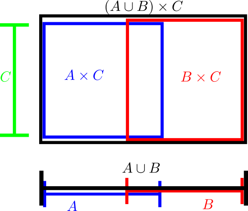
Cartesian product operations can be incorporated into these diagrams by appropriate combinations of one-dimensional and two-dimensional diagrams. Here for instance is a diagram that illustrates the identity {(A \cup B) \times C = (A \times C) \cup (B \times C)}:

cartesian

In this blog post I would like to propose a similar family of diagrams to illustrate relationships between vector spaces (over a fixed base field {k}, such as the reals) or abelian groups, rather than sets. The categories of ({k}-)vector spaces and abelian groups are quite similar in many ways; the former consists of modules over a base field {k}, while the latter consists of modules over the integers {{\bf Z}}; also, both categories are basic examples of abelian categories. The notion of a dimension in a vector space is analogous in many ways to that of cardinality of a set; see this previous post for an instance of this analogy (in the context of Shannon entropy). (UPDATE: I have learned that an essentially identical notation has also been proposed in an unpublished manuscript of Ravi Vakil.)

Read the rest of this entry »

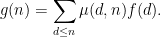
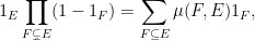
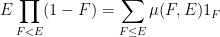
The (classical) Möbius function {\mu: {\bf N} \rightarrow {\bf Z}} is the unique function that obeys the classical Möbius inversion formula:

Proposition 1 (Classical Möbius inversion) Let {f,g: {\bf N} \rightarrow A} be functions from the natural numbers to an additive group {A}. Then the following two claims are equivalent:
  • (i) {f(n) = \sum_{d|n} g(d)} for all {n \in {\bf N}}.
  • (ii) {g(n) = \sum_{d|n} \mu(n/d) f(d)} for all {n \in {\bf N}}.

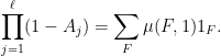
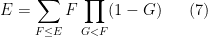
There is a generalisation of this formula to (finite) posets, due to Hall, in which one sums over chains {n_0 > \dots > n_k} in the poset:

Proposition 2 (Poset Möbius inversion) Let {{\mathcal N}} be a finite poset, and let {f,g: {\mathcal N} \rightarrow A} be functions from that poset to an additive group {A}. Then the following two claims are equivalent:
  • (i) {f(n) = \sum_{d \leq n} g(d)} for all {n \in {\mathcal N}}, where {d} is understood to range in {{\mathcal N}}.
  • (ii) {g(n) = \sum_{k=0}^\infty (-1)^k \sum_{n = n_0 > n_1 > \dots > n_k} f(n_k)} for all {n \in {\mathcal N}}, where in the inner sum {n_0,\dots,n_k} are understood to range in {{\mathcal N}} with the indicated ordering.
(Note from the finite nature of {{\mathcal N}} that the inner sum in (ii) is vacuous for all but finitely many {k}.)

Comparing Proposition 2 with Proposition 1, it is natural to refer to the function {\mu(d,n) := \sum_{k=0}^\infty (-1)^k \sum_{n = n_0 > n_1 > \dots > n_k = d} 1} as the Möbius function of the poset; the condition (ii) can then be written as

\displaystyle  g(n) = \sum_{d \leq n} \mu(d,n) f(d).

Proof: If (i) holds, then we have

\displaystyle  g(n) = f(n) - \sum_{d<n} g(d) \ \ \ \ \ (1)

for any {n \in {\mathcal N}}
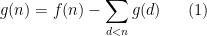
. Iterating this we obtain (ii). Conversely, from (ii) and separating out the {k=0} term, and grouping all the other terms based on the value of {d:=n_1}, we obtain (1), and hence (i). \Box

In fact it is not completely necessary that the poset {{\mathcal N}} be finite; an inspection of the proof shows that it suffices that every element {n} of the poset has only finitely many predecessors {\{ d \in {\mathcal N}: d < n \}}.

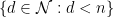
It is not difficult to see that Proposition 2 includes Proposition 1 as a special case, after verifying the combinatorial fact that the quantity

\displaystyle  \sum_{k=0}^\infty (-1)^k \sum_{d=n_k | n_{k-1} | \dots | n_1 | n_0 = n} 1

is equal to {\mu(n/d)} when {d} divides {n}, and vanishes otherwise.

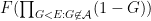
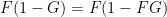
I recently discovered that Proposition 2 can also lead to a useful variant of the inclusion-exclusion principle. The classical version of this principle can be phrased in terms of indicator functions: if
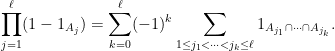
 {A_1,\dots,A_\ell} are subsets of some set {X}, then

\displaystyle  \prod_{j=1}^\ell (1-1_{A_j}) = \sum_{k=0}^\ell (-1)^k \sum_{1 \leq j_1 < \dots < j_k \leq \ell} 1_{A_{j_1} \cap \dots \cap A_{j_k}}.

In particular, if there is a finite measure {\nu} on {X} for which {A_1,\dots,A_\ell} are all measurable, we have

\displaystyle  \nu(X \backslash \bigcup_{j=1}^\ell A_j) = \sum_{k=0}^\ell (-1)^k \sum_{1 \leq j_1 < \dots < j_k \leq \ell} \nu( A_{j_1} \cap \dots \cap A_{j_k} ).

One drawback of this formula is that there are exponentially many terms on the right-hand side: {2^\ell} of them, in fact. However, in many cases of interest there are “collisions” between the intersections {A_{j_1} \cap \dots \cap A_{j_k}} (for instance, perhaps many of the pairwise intersections {A_i \cap A_j} agree), in which case there is an opportunity to collect terms and hopefully achieve some cancellation. It turns out that it is possible to use Proposition 2 to do this, in which one only needs to sum over chains in the resulting poset of intersections:

Proposition 3 (Hall-type inclusion-exclusion principle) Let {A_1,\dots,A_\ell} be subsets of some set {X}, and let {{\mathcal N}} be the finite poset formed by intersections of some of the {A_i} (with the convention that {X} is the empty intersection), ordered by set inclusion. Then for any {E \in {\mathcal N}}, one has

\displaystyle  1_E \prod_{F \subsetneq E} (1 - 1_F) = \sum_{k=0}^\ell (-1)^k \sum_{E = E_0 \supsetneq E_1 \supsetneq \dots \supsetneq E_k} 1_{E_k} \ \ \ \ \ (2)

where {F, E_0,\dots,E_k} are understood to range in {{\mathcal N}}. In particular (setting {E} to be the empty intersection) if the {A_j} are all proper subsets of {X} then we have

\displaystyle  \prod_{j=1}^\ell (1-1_{A_j}) = \sum_{k=0}^\ell (-1)^k \sum_{X = E_0 \supsetneq E_1 \supsetneq \dots \supsetneq E_k} 1_{E_k}. \ \ \ \ \ (3)

In particular, if there is a finite measure {\nu} on {X} for which {A_1,\dots,A_\ell} are all measurable, we have

\displaystyle  \mu(X \backslash \bigcup_{j=1}^\ell A_j) = \sum_{k=0}^\ell (-1)^k \sum_{X = E_0 \supsetneq E_1 \supsetneq \dots \supsetneq E_k} \mu(E_k).

Using the Möbius function {\mu} on the poset {{\mathcal N}}, one can write these formulae as

\displaystyle  1_E \prod_{F \subsetneq E} (1 - 1_F) = \sum_{F \subseteq E} \mu(F,E) 1_F,

\displaystyle  \prod_{j=1}^\ell (1-1_{A_j}) = \sum_F \mu(F,X) 1_F

and

\displaystyle  \nu(X \backslash \bigcup_{j=1}^\ell A_j) = \sum_F \mu(F,X) \nu(F).

Proof: It suffices to establish (2) (to derive (3) from (2) observe that all the {F \subsetneq X} are contained in one of the {A_j}, so the effect of {1-1_F} may be absorbed into {1 - 1_{A_j}}). Applying Proposition 2, this is equivalent to the assertion that

\displaystyle  1_E = \sum_{F \subseteq E} 1_F \prod_{G \subsetneq F} (1 - 1_G)

for all {E \in {\mathcal N}}. But this amounts to the assertion that for each {x \in E}, there is precisely one {F \subseteq E} in {{\mathcal n}} with the property that {x \in F} and {x \not \in G} for any {G \subsetneq F} in {{\mathcal N}}, namely one can take {F} to be the intersection of all {G \subseteq E} in {{\mathcal N}} such that {G} contains {x}. \Box

Example 4 If {A_1,A_2,A_3 \subsetneq X} with {A_1 \cap A_2 = A_1 \cap A_3 = A_2 \cap A_3 = A_*}, and {A_1,A_2,A_3,A_*} are all distinct, then we have for any finite measure {\nu} on {X} that makes {A_1,A_2,A_3} measurable that

\displaystyle  \nu(X \backslash (A_1 \cup A_2 \cup A_3)) = \nu(X) - \nu(A_1) - \nu(A_2) \ \ \ \ \ (4)

\displaystyle  - \nu(A_3) - \nu(A_*) + 3 \nu(A_*)

due to the four chains {X \supsetneq A_1}, {X \supsetneq A_2}, {X \supsetneq A_3}, {X \supsetneq A_*} of length one, and the three chains {X \supsetneq A_1 \supsetneq A_*}, {X \supsetneq A_2 \supsetneq A_*}, {X \supsetneq A_3 \supsetneq A_*} of length two. Note that this expansion just has six terms in it, as opposed to the {2^3=8} given by the usual inclusion-exclusion formula, though of course one can reduce the number of terms by combining the {\nu(A_*)} factors. This may not seem particularly impressive, especially if one views the term {3 \mu(A_*)} as really being three terms instead of one, but if we add a fourth set {A_4 \subsetneq X} with {A_i \cap A_j = A_*} for all {1 \leq i < j \leq 4}, the formula now becomes

\displaystyle  \nu(X \backslash (A_1 \cup A_2 \cup A_3 \cap A_4)) = \nu(X) - \nu(A_1) - \nu(A_2) \ \ \ \ \ (5)

\displaystyle  - \nu(A_3) - \nu(A_4) - \nu(A_*) + 4 \nu(A_*)

and we begin to see more cancellation as we now have just seven terms (or ten if we count {4 \nu(A_*)} as four terms) instead of {2^4 = 16} terms.

Example 5 (Variant of Legendre sieve) If {q_1,\dots,q_\ell > 1} are natural numbers, and {a_1,a_2,\dots} is some sequence of complex numbers with only finitely many terms non-zero, then by applying the above proposition to the sets {A_j := q_j {\bf N}} and with {\nu} equal to counting measure weighted by the {a_n} we obtain a variant of the Legendre sieve

\displaystyle  \sum_{n: (n,q_1 \dots q_\ell) = 1} a_n = \sum_{k=0}^\ell (-1)^k \sum_{1 |' d_1 |' \dots |' d_k} \sum_{n: d_k |n} a_n

where {d_1,\dots,d_k} range over the set {{\mathcal N}} formed by taking least common multiples of the {q_j} (with the understanding that the empty least common multiple is {1}), and {d |' n} denotes the assertion that
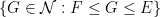
 {d} divides {n} but is strictly less than {n}. I am curious to know of this version of the Legendre sieve already appears in the literature (and similarly for the other applications of Proposition 2 given here).

If the poset {{\mathcal N}} has bounded depth then the number of terms in Proposition 3 can end up being just polynomially large in {\ell} rather than exponentially large. Indeed, if all chains {X \supsetneq E_1 \supsetneq \dots \supsetneq E_k} in {{\mathcal N}} have length {k} at most {k_0} then the number of terms here is at most {1 + \ell + \dots + \ell^{k_0}}. (The examples (4), (5) are ones in which the depth is equal to two.) I hope to report in a later post on how this version of inclusion-exclusion with polynomially many terms can be useful in an application.

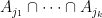
Actually in our application we need an abstraction of the above formula, in which the indicator functions are replaced by more abstract idempotents:

Proposition 6 (Hall-type inclusion-exclusion principle for idempotents) Let {A_1,\dots,A_\ell} be pairwise commuting elements of some ring {R} with identity, which are all idempotent (thus {A_j A_j = A_j} for {j=1,\dots,\ell}). Let {{\mathcal N}} be the finite poset formed by products of the {A_i} (with the convention that {1} is the empty product), ordered by declaring {E \leq F} when {EF = E} (note that all the elements of {{\mathcal N}} are idempotent so this is a partial ordering). Then for any {E \in {\mathcal N}}, one has

\displaystyle  E \prod_{F < E} (1-F) = \sum_{k=0}^\ell (-1)^k \sum_{E = E_0 > E_1 > \dots > E_k} E_k. \ \ \ \ \ (6)

where {F, E_0,\dots,E_k} are understood to range in {{\mathcal N}}. In particular (setting {E=1}) if all the {A_j} are not equal to {1} then we have

\displaystyle  \prod_{j=1}^\ell (1-A_j) = \sum_{k=0}^\ell (-1)^k \sum_{1 = E_0 > E_1 > \dots > E_k} E_k.

Morally speaking this proposition is equivalent to the previous one after applying a “spectral theorem” to simultaneously diagonalise all of the {A_j}, but it is quicker to just adapt the previous proof to establish this proposition directly. Using the Möbius function {\mu} for {{\mathcal N}}, we can rewrite these formulae as

\displaystyle  E \prod_{F < E} (1-F) = \sum_{F \leq E} \mu(F,E) 1_F

and

\displaystyle  \prod_{j=1}^\ell (1-A_j) = \sum_F \mu(F,1) 1_F.

Proof: Again it suffices to verify (6). Using Proposition 2 as before, it suffices to show that

\displaystyle  E = \sum_{F \leq E} F \prod_{G < F} (1 - G) \ \ \ \ \ (7)

for all {E \in {\mathcal N}} (all sums and products are understood to range in {{\mathcal N}}). We can expand

\displaystyle  E = E \prod_{G < E} (G + (1-G)) = \sum_{{\mathcal A}} (\prod_{G \in {\mathcal A}} G) (\prod_{G < E: G \not \in {\mathcal A}} (1-G)) \ \ \ \ \ (8)

where {{\mathcal A}} ranges over all subsets of {\{ G \in {\mathcal N}: G \leq E \}} that contain {E}. For such an {{\mathcal A}}, if we write {F := \prod_{G \in {\mathcal A}} G}, then {F} is the greatest lower bound of {{\mathcal A}}, and we observe that {F (\prod_{G < E: G \not \in {\mathcal A}} (1-G))} vanishes whenever {{\mathcal A}} fails to contain some {G \in {\mathcal N}} with {F \leq G \leq E}. Thus the only {{\mathcal A}} that give non-zero contributions to (8) are the intervals of the form {\{ G \in {\mathcal N}: F \leq G \leq E\}} for some {F \leq E} (which then forms the greatest lower bound for that interval), and the claim (7) follows (after noting that {F (1-G) = F (1-FG)} for any {F,G \in {\mathcal N}}). \Box

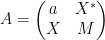
Peter Denton, Stephen Parke, Xining Zhang, and I have just uploaded to the arXiv a completely rewritten version of our previous paper, now titled “Eigenvectors from Eigenvalues: a survey of a basic identity in linear algebra“. This paper is now a survey of the various literature surrounding the following basic identity in linear algebra, which we propose to call the eigenvector-eigenvalue identity:

Theorem 1 (Eigenvector-eigenvalue identity) Let {A} be an {n \times n} Hermitian matrix, with eigenvalues {\lambda_1(A),\dots,\lambda_n(A)}. Let {v_i} be a unit eigenvector corresponding to the eigenvalue {\lambda_i(A)}, and let {v_{i,j}} be the {j^{th}} component of {v_i}. Then

\displaystyle |v_{i,j}|^2 \prod_{k=1; k \neq i}^n (\lambda_i(A) - \lambda_k(A)) = \prod_{k=1}^{n-1} (\lambda_i(A) - \lambda_k(M_j))

where {M_j} is the {n-1 \times n-1} Hermitian matrix formed by deleting the {j^{th}} row and column from {A}.

When we posted the first version of this paper, we were unaware of previous appearances of this identity in the literature; a related identity had been used by Erdos-Schlein-Yau and by myself and Van Vu for applications to random matrix theory, but to our knowledge this specific identity appeared to be new. Even two months after our preprint first appeared on the arXiv in August, we had only learned of one other place in the literature where the identity showed up (by Forrester and Zhang, who also cite an earlier paper of Baryshnikov).

The situation changed rather dramatically with the publication of a popular science article in Quanta on this identity in November, which gave this result significantly more exposure. Within a few weeks we became informed (through private communication, online discussion, and exploration of the citation tree around the references we were alerted to) of over three dozen places where the identity, or some other closely related identity, had previously appeared in the literature, in such areas as numerical linear algebra, various aspects of graph theory (graph reconstruction, chemical graph theory, and walks on graphs), inverse eigenvalue problems, random matrix theory, and neutrino physics. As a consequence, we have decided to completely rewrite our article in order to collate this crowdsourced information, and survey the history of this identity, all the known proofs (we collect seven distinct ways to prove the identity (or generalisations thereof)), and all the applications of it that we are currently aware of. The citation graph of the literature that this ad hoc crowdsourcing effort produced is only very weakly connected, which we found surprising:

The earliest explicit appearance of the eigenvector-eigenvalue identity we are now aware of is in a 1966 paper of Thompson, although this paper is only cited (directly or indirectly) by a fraction of the known literature, and also there is a precursor identity of Löwner from 1934 that can be shown to imply the identity as a limiting case. At the end of the paper we speculate on some possible reasons why this identity only achieved a modest amount of recognition and dissemination prior to the November 2019 Quanta article.

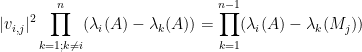
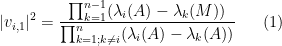
Peter Denton, Stephen Parke, Xining Zhang, and I have just uploaded to the arXiv the short unpublished note “Eigenvectors from eigenvalues“. This note gives two proofs of a general eigenvector identity observed recently by Denton, Parke and Zhang in the course of some quantum mechanical calculations. The identity is as follows:

Theorem 1 Let {A} be an {n \times n} Hermitian matrix, with eigenvalues {\lambda_1(A),\dots,\lambda_n(A)}. Let {v_i} be a unit eigenvector corresponding to the eigenvalue {\lambda_i(A)}, and let {v_{i,j}} be the {j^{th}} component of {v_i}. Then

\displaystyle  |v_{i,j}|^2 \prod_{k=1; k \neq i}^n (\lambda_i(A) - \lambda_k(A)) = \prod_{k=1}^{n-1} (\lambda_i(A) - \lambda_k(M_j))

where {M_j} is the {n-1 \times n-1} Hermitian matrix formed by deleting the {j^{th}} row and column from {A}.

For instance, if we have

\displaystyle  A = \begin{pmatrix} a & X^* \\ X & M \end{pmatrix}

for some real number {a}, {n-1}-dimensional vector {X}, and {n-1 \times n-1} Hermitian matrix {M}, then we have

\displaystyle  |v_{i,1}|^2 = \frac{\prod_{k=1}^{n-1} (\lambda_i(A) - \lambda_k(M))}{\prod_{k=1; k \neq i}^n (\lambda_i(A) - \lambda_k(A))} \ \ \ \ \ (1)

assuming that the denominator is non-zero.

Once one is aware of the identity, it is not so difficult to prove it; we give two proofs, each about half a page long, one of which is based on a variant of the Cauchy-Binet formula, and the other based on properties of the adjugate matrix. But perhaps it is surprising that such a formula exists at all; one does not normally expect to learn much information about eigenvectors purely from knowledge of eigenvalues. In the random matrix theory literature, for instance in this paper of Erdos, Schlein, and Yau, or this later paper of Van Vu and myself, a related identity has been used, namely

\displaystyle  |v_{i,1}|^2 = \frac{1}{1 + \| (M-\lambda_i(A))^{-1} X \|^2}, \ \ \ \ \ (2)

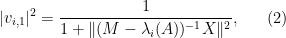
but it is not immediately obvious that one can derive the former identity from the latter. (I do so below the fold; we ended up not putting this proof in the note as it was longer than the two other proofs we found. I also give two other proofs below the fold, one from a more geometric perspective and one proceeding via Cramer’s rule.) It was certainly something of a surprise to me that there is no explicit appearance of the {a,X} components of {A} in the formula (1) (though they do indirectly appear through their effect on the eigenvalues {\lambda_k(A)}; for instance from taking traces one sees that {a = \sum_{k=1}^n \lambda_k(A) - \sum_{k=1}^{n-1} \lambda_k(M)}).

One can get some feeling of the identity (1) by considering some special cases. Suppose for instance that {A} is a diagonal matrix with all distinct entries. The upper left entry {a} of {A} is one of the eigenvalues of {A}. If it is equal to {\lambda_i(A)}, then the eigenvalues of {M} are the other {n-1} eigenvalues of {A}, and now the left and right-hand sides of (1) are equal to {1}. At the other extreme, if {a} is equal to a different eigenvalue of {A}, then {\lambda_i(A)} now appears as an eigenvalue of {M}, and both sides of (1) now vanish. More generally, if we order the eigenvalues {\lambda_1(A) \leq \dots \leq \lambda_n(A)} and {\lambda_1(M) \leq \dots \leq \lambda_{n-1}(M)}, then the Cauchy interlacing inequalities tell us that

\displaystyle  0 \leq \lambda_i(A) - \lambda_k(M) \leq \lambda_i(A) - \lambda_k(A)

for {1 \leq k < i}, and

\displaystyle  \lambda_i(A) - \lambda_{k+1}(A) \leq \lambda_i(A) - \lambda_k(M) < 0

for {i \leq k \leq n-1}, so that the right-hand side of (1) lies between {0} and {1}, which is of course consistent with (1) as {v_i} is a unit vector. Thus the identity relates the coefficient sizes of an eigenvector with the extent to which the Cauchy interlacing inequalities are sharp.

Read the rest of this entry »

(This post is mostly intended for my own reference, as I found myself repeatedly looking up several conversions between polynomial bases on various occasions.)

Let {\mathrm{Poly}_{\leq n}} denote the vector space of polynomials {P:{\bf R} \rightarrow {\bf R}} of one variable {x} with real coefficients of degree at most {n}. This is a vector space of dimension {n+1}, and the sequence of these spaces form a filtration:

\displaystyle  \mathrm{Poly}_{\leq 0} \subset \mathrm{Poly}_{\leq 1} \subset \mathrm{Poly}_{\leq 2} \subset \dots

A standard basis for these vector spaces are given by the monomials {x^0, x^1, x^2, \dots}: every polynomial {P(x)} in {\mathrm{Poly}_{\leq n}} can be expressed uniquely as a linear combination of the first {n+1} monomials {x^0, x^1, \dots, x^n}. More generally, if one has any sequence {Q_0(x), Q_1(x), Q_2(x)} of polynomials, with each {Q_n} of degree exactly {n}, then an easy induction shows that {Q_0(x),\dots,Q_n(x)} forms a basis for {\mathrm{Poly}_{\leq n}}.

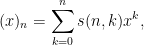
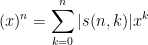
In particular, if we have two such sequences {Q_0(x), Q_1(x), Q_2(x),\dots} and {R_0(x), R_1(x), R_2(x), \dots} of polynomials, with each {Q_n} of degree {n} and each {R_k} of degree {k}, then {Q_n} must be expressible uniquely as a linear combination of the polynomials {R_0,R_1,\dots,R_n}, thus we have an identity of the form

\displaystyle  Q_n(x) = \sum_{k=0}^n c_{QR}(n,k) R_k(x)

for some change of basis coefficients {c_{QR}(n,k) \in {\bf R}}. These coefficients describe how to convert a polynomial expressed in the {Q_n} basis into a polynomial expressed in the {R_k} basis.

Many standard combinatorial quantities {c(n,k)} involving two natural numbers {0 \leq k \leq n} can be interpreted as such change of basis coefficients. The most familiar example are the binomial coefficients {\binom{n}{k}}, which measures the conversion from the shifted monomial basis {(x+1)^n} to the monomial basis {x^k}, thanks to (a special case of) the binomial formula:

\displaystyle  (x+1)^n = \sum_{k=0}^n \binom{n}{k} x^k,

thus for instance

\displaystyle  (x+1)^3 = \binom{3}{0} x^0 + \binom{3}{1} x^1 + \binom{3}{2} x^2 + \binom{3}{3} x^3

\displaystyle  = 1 + 3x + 3x^2 + x^3.

More generally, for any shift {h}, the conversion from {(x+h)^n} to {x^k} is measured by the coefficients {h^{n-k} \binom{n}{k}}, thanks to the general case of the binomial formula.

But there are other bases of interest too. For instance if one uses the falling factorial basis

\displaystyle  (x)_n := x (x-1) \dots (x-n+1)

then the conversion from falling factorials to monomials is given by the Stirling numbers of the first kind {s(n,k)}:

\displaystyle  (x)_n = \sum_{k=0}^n s(n,k) x^k,

thus for instance

\displaystyle  (x)_3 = s(3,0) x^0 + s(3,1) x^1 + s(3,2) x^2 + s(3,3) x^3

\displaystyle  = 0 + 2 x - 3x^2 + x^3

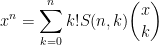
and the conversion back is given by the Stirling numbers of the second kind {S(n,k)}:

\displaystyle  x^n = \sum_{k=0}^n S(n,k) (x)_k

thus for instance

\displaystyle  x^3 = S(3,0) (x)_0 + S(3,1) (x)_1 + S(3,2) (x)_2 + S(3,3) (x)_3

\displaystyle  = 0 + x + 3 x(x-1) + x(x-1)(x-2).

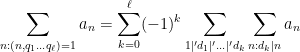
If one uses the binomial functions {\binom{x}{n} = \frac{1}{n!} (x)_n} as a basis instead of the falling factorials, one of course can rewrite these conversions as

\displaystyle  \binom{x}{n} = \sum_{k=0}^n \frac{1}{n!} s(n,k) x^k

and

\displaystyle  x^n = \sum_{k=0}^n k! S(n,k) \binom{x}{k}

thus for instance

\displaystyle  \binom{x}{3} = 0 + \frac{1}{3} x - \frac{1}{2} x^2 + \frac{1}{6} x^3

and

\displaystyle  x^3 = 0 + \binom{x}{1} + 6 \binom{x}{2} + 6 \binom{x}{3}.

As a slight variant, if one instead uses rising factorials

\displaystyle  (x)^n := x (x+1) \dots (x+n-1)

then the conversion to monomials yields the unsigned Stirling numbers {|s(n,k)|} of the first kind:

\displaystyle  (x)^n = \sum_{k=0}^n |s(n,k)| x^k

thus for instance

\displaystyle  (x)^3 = 0 + 2x + 3x^2 + x^3.

One final basis comes from the polylogarithm functions

\displaystyle  \mathrm{Li}_{-n}(x) := \sum_{j=1}^\infty j^n x^j.

For instance one has

\displaystyle  \mathrm{Li}_1(x) = -\log(1-x)

\displaystyle  \mathrm{Li}_0(x) = \frac{x}{1-x}

\displaystyle  \mathrm{Li}_{-1}(x) = \frac{x}{(1-x)^2}

\displaystyle  \mathrm{Li}_{-2}(x) = \frac{x}{(1-x)^3} (1+x)

\displaystyle  \mathrm{Li}_{-3}(x) = \frac{x}{(1-x)^4} (1+4x+x^2)

\displaystyle  \mathrm{Li}_{-4}(x) = \frac{x}{(1-x)^5} (1+11x+11x^2+x^3)

and more generally one has

\displaystyle  \mathrm{Li}_{-n-1}(x) = \frac{x}{(1-x)^{n+2}} E_n(x)

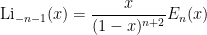
for all natural numbers {n} and some polynomial {E_n} of degree {n} (the Eulerian polynomials), which when converted to the monomial basis yields the (shifted) Eulerian numbers

\displaystyle  E_n(x) = \sum_{k=0}^n A(n+1,k) x^k.

For instance

\displaystyle  E_3(x) = A(4,0) x^0 + A(4,1) x^1 + A(4,2) x^2 + A(4,3) x^3

\displaystyle  = 1 + 11x + 11x^2 + x^3.

These particular coefficients also have useful combinatorial interpretations. For instance:

  • The binomial coefficient {\binom{n}{k}} is of course the number of {k}-element subsets of {\{1,\dots,n\}}.
  • The unsigned Stirling numbers {|s(n,k)|} of the first kind are the number of permutations of {\{1,\dots,n\}} with exactly {k} cycles. The signed Stirling numbers {s(n,k)} are then given by the formula {s(n,k) = (-1)^{n-k} |s(n,k)|}.
  • The Stirling numbers {S(n,k)} of the second kind are the number of ways to partition {\{1,\dots,n\}} into {k} non-empty subsets.
  • The Eulerian numbers {A(n,k)} are the number of permutations of {\{1,\dots,n\}} with exactly {k} ascents.

These coefficients behave similarly to each other in several ways. For instance, the binomial coefficients {\binom{n}{k}} obey the well known Pascal identity

\displaystyle  \binom{n+1}{k} = \binom{n}{k} + \binom{n}{k-1}

(with the convention that {\binom{n}{k}} vanishes outside of the range {0 \leq k \leq n}). In a similar spirit, the unsigned Stirling numbers {|s(n,k)|} of the first kind obey the identity

\displaystyle  |s(n+1,k)| = n |s(n,k)| + |s(n,k-1)|

and the signed counterparts {s(n,k)} obey the identity

\displaystyle  s(n+1,k) = -n s(n,k) + s(n,k-1).

The Stirling numbers of the second kind {S(n,k)} obey the identity

\displaystyle  S(n+1,k) = k S(n,k) + S(n,k-1)

and the Eulerian numbers {A(n,k)} obey the identity

\displaystyle  A(n+1,k) = (k+1) A(n,k) + (n-k+1) A(n,k-1).

While talking mathematics with a postdoc here at UCLA (March Boedihardjo) we came across the following matrix problem which we managed to solve, but the proof was cute and the process of discovering it was fun, so I thought I would present the problem here as a puzzle without revealing the solution for now.

The problem involves word maps on a matrix group, which for sake of discussion we will take to be the special orthogonal group SO(3) of real 3 \times 3 matrices (one of the smallest matrix groups that contains a copy of the free group, which incidentally is the key observation powering the Banach-Tarski paradox).  Given any abstract word w of two generators x,y and their inverses (i.e., an element of the free group {\bf F}_2), one can define the word map w: SO(3) \times SO(3) \to SO(3) simply by substituting a pair of matrices in SO(3) into these generators.  For instance, if one has the word w = x y x^{-2} y^2 x, then the corresponding word map w: SO(3) \times SO(3) \to SO(3) is given by

\displaystyle w(A,B) := ABA^{-2} B^2 A

for A,B \in SO(3).  Because SO(3) contains a copy of the free group, we see the word map is non-trivial (not equal to the identity) if and only if the word itself is nontrivial.

Anyway, here is the problem:

Problem. Does there exist a sequence w_1, w_2, \dots of non-trivial word maps w_n: SO(3) \times SO(3) \to SO(3) that converge uniformly to the identity map?

To put it another way, given any \varepsilon > 0, does there exist a non-trivial word w such that \|w(A,B) - 1 \| \leq \varepsilon for all A,B \in SO(3), where \| \| denotes (say) the operator norm, and 1 denotes the identity matrix in SO(3)?

As I said, I don’t want to spoil the fun of working out this problem, so I will leave it as a challenge. Readers are welcome to share their thoughts, partial solutions, or full solutions in the comments below.

Apoorva Khare and I have updated our paper “On the sign patterns of entrywise positivity preservers in fixed dimension“, announced at this post from last month. The quantitative results are now sharpened using a new monotonicity property of ratios {s_{\lambda}(u)/s_{\mu}(u)} of Schur polynomials, namely that such ratios are monotone non-decreasing in each coordinate of {u} if {u} is in the positive orthant, and the partition {\lambda} is larger than that of {\mu}. (This monotonicity was also independently observed by Rachid Ait-Haddou, using the theory of blossoms.) In the revised version of the paper we give two proofs of this monotonicity. The first relies on a deep positivity result of Lam, Postnikov, and Pylyavskyy, which uses a representation-theoretic positivity result of Haiman to show that the polynomial combination

\displaystyle s_{(\lambda \wedge \nu) / (\mu \wedge \rho)} s_{(\lambda \vee \nu) / (\mu \vee \rho)} - s_{\lambda/\mu} s_{\nu/\rho} \ \ \ \ \ (1)

of skew-Schur polynomials is Schur-positive for any partitions {\lambda,\mu,\nu,\rho} (using the convention that the skew-Schur polynomial {s_{\lambda/\mu}} vanishes if {\mu} is not contained in {\lambda}, and where {\lambda \wedge \nu} and {\lambda \vee \nu} denotes the pointwise min and max of {\lambda} and {\nu} respectively). It is fairly easy to derive the monotonicity of {s_\lambda(u)/s_\mu(u)} from this, by using the expansion

\displaystyle s_\lambda(u_1,\dots, u_n) = \sum_k u_1^k s_{\lambda/(k)}(u_2,\dots,u_n)

of Schur polynomials into skew-Schur polynomials (as was done in this previous post).

The second proof of monotonicity avoids representation theory by a more elementary argument establishing the weaker claim that the above expression (1) is non-negative on the positive orthant. In fact we prove a more general determinantal log-supermodularity claim which may be of independent interest:

Theorem 1 Let {A} be any {n \times n} totally positive matrix (thus, every minor has a non-negative determinant). Then for any {k}-tuples {I_1,I_2,J_1,J_2} of increasing elements of {\{1,\dots,n\}}, one has

\displaystyle \det( A_{I_1 \wedge I_2, J_1 \wedge J_2} ) \det( A_{I_1 \vee I_2, J_1 \vee J_2} ) - \det(A_{I_1,J_1}) \det(A_{I_2,J_2}) \geq 0

where {A_{I,J}} denotes the {k \times k} minor formed from the rows in {I} and columns in {J}.

For instance, if {A} is the matrix

\displaystyle A = \begin{pmatrix} a & b & c & d \\ e & f & g & h \\ i & j & k & l \\ m & n & o & p \end{pmatrix}

for some real numbers {a,\dots,p}, one has

\displaystyle a h - de\geq 0

(corresponding to the case {k=1}, {I_1 = (1), I_2 = (2), J_1 = (4), J_2 = (1)}), or

\displaystyle \det \begin{pmatrix} a & c \\ i & k \end{pmatrix} \det \begin{pmatrix} f & h \\ n & p \end{pmatrix} - \det \begin{pmatrix} e & h \\ i & l \end{pmatrix} \det \begin{pmatrix} b & c \\ n & o \end{pmatrix} \geq 0

(corresponding to the case {k=2}, {I_1 = (2,3)}, {I_2 = (1,4)}, {J_1 = (1,4)}, {J_2 = (2,3)}). It turns out that this claim can be proven relatively easy by an induction argument, relying on the Dodgson and Karlin identities from this previous post; the difficulties are largely notational in nature. Combining this result with the Jacobi-Trudi identity for skew-Schur polynomials (discussed in this previous post) gives the non-negativity of (1); it can also be used to directly establish the monotonicity of ratios {s_\lambda(u)/s_\mu(u)} by applying the theorem to a generalised Vandermonde matrix.

(Log-supermodularity also arises as the natural hypothesis for the FKG inequality, though I do not know of any interesting application of the FKG inequality in this current setting.)

Suppose we have an {n \times n} matrix {M} that is expressed in block-matrix form as

\displaystyle  M = \begin{pmatrix} A & B \\ C & D \end{pmatrix}

where {A} is an {(n-k) \times (n-k)} matrix, {B} is an {(n-k) \times k} matrix, {C} is an {k \times (n-k)} matrix, and {D} is a {k \times k} matrix for some {1 < k < n}. If {A} is invertible, we can use the technique of Schur complementation to express the inverse of {M} (if it exists) in terms of the inverse of {A}, and the other components {B,C,D} of course. Indeed, to solve the equation

\displaystyle  M \begin{pmatrix} x & y \end{pmatrix} = \begin{pmatrix} a & b \end{pmatrix},

where {x, a} are {(n-k) \times 1} column vectors and {y,b} are {k \times 1} column vectors, we can expand this out as a system

\displaystyle  Ax + By = a

\displaystyle  Cx + Dy = b.

Using the invertibility of {A}, we can write the first equation as

\displaystyle  x = A^{-1} a - A^{-1} B y \ \ \ \ \ (1)

and substituting this into the second equation yields

\displaystyle  (D - C A^{-1} B) y = b - C A^{-1} a

and thus (assuming that {D - CA^{-1} B} is invertible)

\displaystyle  y = - (D - CA^{-1} B)^{-1} CA^{-1} a + (D - CA^{-1} B)^{-1} b

and then inserting this back into (1) gives

\displaystyle  x = (A^{-1} + A^{-1} B (D - CA^{-1} B)^{-1} C A^{-1}) a - A^{-1} B (D - CA^{-1} B)^{-1} b.

Comparing this with

\displaystyle  \begin{pmatrix} x & y \end{pmatrix} = M^{-1} \begin{pmatrix} a & b \end{pmatrix},

we have managed to express the inverse of {M} as

\displaystyle  M^{-1} =

\displaystyle  \begin{pmatrix} A^{-1} + A^{-1} B (D - CA^{-1} B)^{-1} C A^{-1} & - A^{-1} B (D - CA^{-1} B)^{-1} \\ - (D - CA^{-1} B)^{-1} CA^{-1} & (D - CA^{-1} B)^{-1} \end{pmatrix}. \ \ \ \ \ (2)

One can consider the inverse problem: given the inverse {M^{-1}} of {M}, does one have a nice formula for the inverse {A^{-1}} of the minor {A}? Trying to recover this directly from (2) looks somewhat messy. However, one can proceed as follows. Let {U} denote the {n \times k} matrix

\displaystyle  U := \begin{pmatrix} 0 \\ I_k \end{pmatrix}

(with {I_k} the {k \times k} identity matrix), and let {V} be its transpose:

\displaystyle  V := \begin{pmatrix} 0 & I_k \end{pmatrix}.

Then for any scalar {t} (which we identify with {t} times the identity matrix), one has

\displaystyle  M + UtV = \begin{pmatrix} A & B \\ C & D+t \end{pmatrix},

and hence by (2)

\displaystyle  (M+UtV)^{-1} =

\displaystyle \begin{pmatrix} A^{-1} + A^{-1} B (D + t - CA^{-1} B)^{-1} C A^{-1} & - A^{-1} B (D + t- CA^{-1} B)^{-1} \\ - (D + t - CA^{-1} B)^{-1} CA^{-1} & (D + t - CA^{-1} B)^{-1} \end{pmatrix}.

noting that the inverses here will exist for {t} large enough. Taking limits as {t \rightarrow \infty}, we conclude that

\displaystyle  \lim_{t \rightarrow \infty} (M+UtV)^{-1} = \begin{pmatrix} A^{-1} & 0 \\ 0 & 0 \end{pmatrix}.

On the other hand, by the Woodbury matrix identity (discussed in this previous blog post), we have

\displaystyle  (M+UtV)^{-1} = M^{-1} - M^{-1} U (t^{-1} + V M^{-1} U)^{-1} V M^{-1}

and hence on taking limits and comparing with the preceding identity, one has

\displaystyle  \begin{pmatrix} A^{-1} & 0 \\ 0 & 0 \end{pmatrix} = M^{-1} - M^{-1} U (V M^{-1} U)^{-1} V M^{-1}.

This achieves the aim of expressing the inverse {A^{-1}} of the minor in terms of the inverse of the full matrix. Taking traces and rearranging, we conclude in particular that

\displaystyle  \mathrm{tr} A^{-1} = \mathrm{tr} M^{-1} - \mathrm{tr} (V M^{-2} U) (V M^{-1} U)^{-1}. \ \ \ \ \ (3)

In the {k=1} case, this can be simplified to

\displaystyle  \mathrm{tr} A^{-1} = \mathrm{tr} M^{-1} - \frac{e_n^T M^{-2} e_n}{e_n^T M^{-1} e_n} \ \ \ \ \ (4)

where {e_n} is the {n^{th}} basis column vector.

We can apply this identity to understand how the spectrum of an {n \times n} random matrix {M} relates to that of its top left {n-1 \times n-1} minor {A}. Subtracting any complex multiple {z} of the identity from {M} (and hence from {A}), we can relate the Stieltjes transform {s_M(z) := \frac{1}{n} \mathrm{tr}(M-z)^{-1}} of {M} with the Stieltjes transform {s_A(z) := \frac{1}{n-1} \mathrm{tr}(A-z)^{-1}} of {A}:

\displaystyle  s_A(z) = \frac{n}{n-1} s_M(z) - \frac{1}{n-1} \frac{e_n^T (M-z)^{-2} e_n}{e_n^T (M-z)^{-1} e_n} \ \ \ \ \ (5)

At this point we begin to proceed informally. Assume for sake of argument that the random matrix {M} is Hermitian, with distribution that is invariant under conjugation by the unitary group {U(n)}; for instance, {M} could be drawn from the Gaussian Unitary Ensemble (GUE), or alternatively {M} could be of the form {M = U D U^*} for some real diagonal matrix {D} and {U} a unitary matrix drawn randomly from {U(n)} using Haar measure. To fix normalisations we will assume that the eigenvalues of {M} are typically of size {O(1)}. Then {A} is also Hermitian and {U(n)}-invariant. Furthermore, the law of {e_n^T (M-z)^{-1} e_n} will be the same as the law of {u^* (M-z)^{-1} u}, where {u} is now drawn uniformly from the unit sphere (independently of {M}). Diagonalising {M} into eigenvalues {\lambda_j} and eigenvectors {v_j}, we have

\displaystyle u^* (M-z)^{-1} u = \sum_{j=1}^n \frac{|u^* v_j|^2}{\lambda_j - z}.

One can think of {u} as a random (complex) Gaussian vector, divided by the magnitude of that vector (which, by the Chernoff inequality, will concentrate to {\sqrt{n}}). Thus the coefficients {u^* v_j} with respect to the orthonormal basis {v_1,\dots,v_j} can be thought of as independent (complex) Gaussian vectors, divided by that magnitude. Using this and the Chernoff inequality again, we see (for {z} distance {\sim 1} away from the real axis at least) that one has the concentration of measure

\displaystyle  u^* (M-z)^{-1} u \approx \frac{1}{n} \sum_{j=1}^n \frac{1}{\lambda_j - z}

and thus

\displaystyle  e_n^T (M-z)^{-1} e_n \approx \frac{1}{n} \mathrm{tr} (M-z)^{-1} = s_M(z)

(that is to say, the diagonal entries of {(M-z)^{-1}} are roughly constant). Similarly we have

\displaystyle  e_n^T (M-z)^{-2} e_n \approx \frac{1}{n} \mathrm{tr} (M-z)^{-2} = \frac{d}{dz} s_M(z).

Inserting this into (5) and discarding terms of size {O(1/n^2)}, we thus conclude the approximate relationship

\displaystyle  s_A(z) \approx s_M(z) + \frac{1}{n} ( s_M(z) - s_M(z)^{-1} \frac{d}{dz} s_M(z) ).

This can be viewed as a difference equation for the Stieltjes transform of top left minors of {M}. Iterating this equation, and formally replacing the difference equation by a differential equation in the large {n} limit, we see that when {n} is large and {k \approx e^{-t} n} for some {t \geq 0}, one expects the top left {k \times k} minor {A_k} of {M} to have Stieltjes transform

\displaystyle  s_{A_k}(z) \approx s( t, z ) \ \ \ \ \ (6)

where {s(t,z)} solves the Burgers-type equation

\displaystyle  \partial_t s(t,z) = s(t,z) - s(t,z)^{-1} \frac{d}{dz} s(t,z) \ \ \ \ \ (7)

with initial data {s(0,z) = s_M(z)}.

Example 1 If {M} is a constant multiple {M = cI_n} of the identity, then {s_M(z) = \frac{1}{c-z}}. One checks that {s(t,z) = \frac{1}{c-z}} is a steady state solution to (7), which is unsurprising given that all minors of {M} are also {c} times the identity.

Example 2 If {M} is GUE normalised so that each entry has variance {\sigma^2/n}, then by the semi-circular law (see previous notes) one has {s_M(z) \approx \frac{-z + \sqrt{z^2-4\sigma^2}}{2\sigma^2} = -\frac{2}{z + \sqrt{z^2-4\sigma^2}}} (using an appropriate branch of the square root). One can then verify the self-similar solution

\displaystyle  s(t,z) = \frac{-z + \sqrt{z^2 - 4\sigma^2 e^{-t}}}{2\sigma^2 e^{-t}} = -\frac{2}{z + \sqrt{z^2 - 4\sigma^2 e^{-t}}}

to (7), which is consistent with the fact that a top {k \times k} minor of {M} also has the law of GUE, with each entry having variance {\sigma^2 / n \approx \sigma^2 e^{-t} / k} when {k \approx e^{-t} n}.

One can justify the approximation (6) given a sufficiently good well-posedness theory for the equation (7). We will not do so here, but will note that (as with the classical inviscid Burgers equation) the equation can be solved exactly (formally, at least) by the method of characteristics. For any initial position {z_0}, we consider the characteristic flow {t \mapsto z(t)} formed by solving the ODE

\displaystyle  \frac{d}{dt} z(t) = s(t,z(t))^{-1} \ \ \ \ \ (8)

with initial data {z(0) = z_0}, ignoring for this discussion the problems of existence and uniqueness. Then from the chain rule, the equation (7) implies that

\displaystyle  \frac{d}{dt} s( t, z(t) ) = s(t,z(t))

and thus {s(t,z(t)) = e^t s(0,z_0)}. Inserting this back into (8) we see that

\displaystyle  z(t) = z_0 + s(0,z_0)^{-1} (1-e^{-t})

and thus (7) may be solved implicitly via the equation

\displaystyle  s(t, z_0 + s(0,z_0)^{-1} (1-e^{-t}) ) = e^t s(0, z_0) \ \ \ \ \ (9)

for all {t} and {z_0}.

Remark 3 In practice, the equation (9) may stop working when {z_0 + s(0,z_0)^{-1} (1-e^{-t})} crosses the real axis, as (7) does not necessarily hold in this region. It is a cute exercise (ultimately coming from the Cauchy-Schwarz inequality) to show that this crossing always happens, for instance if {z_0} has positive imaginary part then {z_0 + s(0,z_0)^{-1}} necessarily has negative or zero imaginary part.

Example 4 Suppose we have {s(0,z) = \frac{1}{c-z}} as in Example 1. Then (9) becomes

\displaystyle  s( t, z_0 + (c-z_0) (1-e^{-t}) ) = \frac{e^t}{c-z_0}

for any {t,z_0}, which after making the change of variables {z = z_0 + (c-z_0) (1-e^{-t}) = c - e^{-t} (c - z_0)} becomes

\displaystyle  s(t, z ) = \frac{1}{c-z}

as in Example 1.

Example 5 Suppose we have

\displaystyle  s(0,z) = \frac{-z + \sqrt{z^2-4\sigma^2}}{2\sigma^2} = -\frac{2}{z + \sqrt{z^2-4\sigma^2}}.

as in Example 2. Then (9) becomes

\displaystyle  s(t, z_0 - \frac{z_0 + \sqrt{z_0^2-4\sigma^2}}{2} (1-e^{-t}) ) = e^t \frac{-z_0 + \sqrt{z_0^2-4\sigma^2}}{2\sigma^2}.

If we write

\displaystyle  z := z_0 - \frac{z_0 + \sqrt{z_0^2-4\sigma^2}}{2} (1-e^{-t})

\displaystyle  = \frac{(1+e^{-t}) z_0 - (1-e^{-t}) \sqrt{z_0^2-4\sigma^2}}{2}

one can calculate that

\displaystyle  z^2 - 4 \sigma^2 e^{-t} = (\frac{(1-e^{-t}) z_0 - (1+e^{-t}) \sqrt{z_0^2-4\sigma^2}}{2})^2

and hence

\displaystyle  \frac{-z + \sqrt{z^2 - 4\sigma^2 e^{-t}}}{2\sigma^2 e^{-t}} = e^t \frac{-z_0 + \sqrt{z_0^2-4\sigma^2}}{2\sigma^2}

which gives

\displaystyle  s(t,z) = \frac{-z + \sqrt{z^2 - 4\sigma^2 e^{-t}}}{2\sigma^2 e^{-t}}. \ \ \ \ \ (10)

One can recover the spectral measure {\mu} from the Stieltjes transform {s(z)} as the weak limit of {x \mapsto \frac{1}{\pi} \mathrm{Im} s(x+i\varepsilon)} as {\varepsilon \rightarrow 0}; we write this informally as

\displaystyle  d\mu(x) = \frac{1}{\pi} \mathrm{Im} s(x+i0^+)\ dx.

In this informal notation, we have for instance that

\displaystyle  \delta_c(x) = \frac{1}{\pi} \mathrm{Im} \frac{1}{c-x-i0^+}\ dx

which can be interpreted as the fact that the Cauchy distributions {\frac{1}{\pi} \frac{\varepsilon}{(c-x)^2+\varepsilon^2}} converge weakly to the Dirac mass at {c} as {\varepsilon \rightarrow 0}. Similarly, the spectral measure associated to (10) is the semicircular measure {\frac{1}{2\pi \sigma^2 e^{-t}} (4 \sigma^2 e^{-t}-x^2)_+^{1/2}}.

If we let {\mu_t} be the spectral measure associated to {s(t,\cdot)}, then the curve {e^{-t} \mapsto \mu_t} from {(0,1]} to the space of measures is the high-dimensional limit {n \rightarrow \infty} of a Gelfand-Tsetlin pattern (discussed in this previous post), if the pattern is randomly generated amongst all matrices {M} with spectrum asymptotic to {\mu_0} as {n \rightarrow \infty}. For instance, if {\mu_0 = \delta_c}, then the curve is {\alpha \mapsto \delta_c}, corresponding to a pattern that is entirely filled with {c}‘s. If instead {\mu_0 = \frac{1}{2\pi \sigma^2} (4\sigma^2-x^2)_+^{1/2}} is a semicircular distribution, then the pattern is

\displaystyle  \alpha \mapsto \frac{1}{2\pi \sigma^2 \alpha} (4\sigma^2 \alpha -x^2)_+^{1/2},

thus at height {\alpha} from the top, the pattern is semicircular on the interval {[-2\sigma \sqrt{\alpha}, 2\sigma \sqrt{\alpha}]}. The interlacing property of Gelfand-Tsetlin patterns translates to the claim that {\alpha \mu_\alpha(-\infty,\lambda)} (resp. {\alpha \mu_\alpha(\lambda,\infty)}) is non-decreasing (resp. non-increasing) in {\alpha} for any fixed {\lambda}. In principle one should be able to establish these monotonicity claims directly from the PDE (7) or from the implicit solution (9), but it was not clear to me how to do so.

An interesting example of such a limiting Gelfand-Tsetlin pattern occurs when {\mu_0 = \frac{1}{2} \delta_{-1} + \frac{1}{2} \delta_1}, which corresponds to {M} being {2P-I}, where {P} is an orthogonal projection to a random {n/2}-dimensional subspace of {{\bf C}^n}. Here we have

\displaystyle  s(0,z) = \frac{1}{2} \frac{1}{-1-z} + \frac{1}{2} \frac{1}{1-z} = \frac{z}{1-z^2}

and so (9) in this case becomes

\displaystyle  s(t, z_0 + \frac{1-z_0^2}{z_0} (1-e^{-t}) ) = \frac{e^t z_0}{1-z_0^2}

A tedious calculation then gives the solution

\displaystyle  s(t,z) = \frac{(2e^{-t}-1)z + \sqrt{z^2 - 4e^{-t}(1-e^{-t})}}{2e^{-t}(1-z^2)}. \ \ \ \ \ (11)

For {\alpha = e^{-t} > 1/2}, there are simple poles at {z=-1,+1}, and the associated measure is

\displaystyle  \mu_\alpha = \frac{2\alpha-1}{2\alpha} \delta_{-1} + \frac{2\alpha-1}{2\alpha} \delta_1 + \frac{1}{2\pi \alpha(1-x^2)} (4\alpha(1-\alpha)-x^2)_+^{1/2}\ dx.

This reflects the interlacing property, which forces {\frac{2\alpha-1}{2\alpha} \alpha n} of the {\alpha n} eigenvalues of the {\alpha n \times \alpha n} minor to be equal to {-1} (resp. {+1}). For {\alpha = e^{-t} \leq 1/2}, the poles disappear and one just has

\displaystyle  \mu_\alpha = \frac{1}{2\pi \alpha(1-x^2)} (4\alpha(1-\alpha)-x^2)_+^{1/2}\ dx.

For {\alpha=1/2}, one has an inverse semicircle distribution

\displaystyle  \mu_{1/2} = \frac{1}{\pi} (1-x^2)_+^{-1/2}.

There is presumably a direct geometric explanation of this fact (basically describing the singular values of the product of two random orthogonal projections to half-dimensional subspaces of {{\bf C}^n}), but I do not know of one off-hand.

The evolution of {s(t,z)} can also be understood using the {R}-transform and {S}-transform from free probability. Formally, letlet {z(t,s)} be the inverse of {s(t,z)}, thus

\displaystyle  s(t,z(t,s)) = s

for all {t,s}, and then define the {R}-transform

\displaystyle  R(t,s) := z(t,-s) - \frac{1}{s}.

The equation (9) may be rewritten as

\displaystyle  z( t, e^t s ) = z(0,s) + s^{-1} (1-e^{-t})

and hence

\displaystyle  R(t, -e^t s) = R(0, -s)

or equivalently

\displaystyle  R(t,s) = R(0, e^{-t} s). \ \ \ \ \ (12)

See these previous notes for a discussion of free probability topics such as the {R}-transform.

Example 6 If {s(t,z) = \frac{1}{c-z}} then the {R} transform is {R(t,s) = c}.

Example 7 If {s(t,z)} is given by (10), then the {R} transform is

\displaystyle  R(t,s) = \sigma^2 e^{-t} s.

Example 8 If {s(t,z)} is given by (11), then the {R} transform is

\displaystyle  R(t,s) = \frac{-1 + \sqrt{1 + 4 s^2 e^{-2t}}}{2 s e^{-t}}.

This simple relationship (12) is essentially due to Nica and Speicher (thanks to Dima Shylakhtenko for this reference). It has the remarkable consequence that when {\alpha = 1/m} is the reciprocal of a natural number {m}, then {\mu_{1/m}} is the free arithmetic mean of {m} copies of {\mu}, that is to say {\mu_{1/m}} is the free convolution {\mu \boxplus \dots \boxplus \mu} of {m} copies of {\mu}, pushed forward by the map {\lambda \rightarrow \lambda/m}. In terms of random matrices, this is asserting that the top {n/m \times n/m} minor of a random matrix {M} has spectral measure approximately equal to that of an arithmetic mean {\frac{1}{m} (M_1 + \dots + M_m)} of {m} independent copies of {M}, so that the process of taking top left minors is in some sense a continuous analogue of the process of taking freely independent arithmetic means. There ought to be a geometric proof of this assertion, but I do not know of one. In the limit {m \rightarrow \infty} (or {\alpha \rightarrow 0}), the {R}-transform becomes linear and the spectral measure becomes semicircular, which is of course consistent with the free central limit theorem.

In a similar vein, if one defines the function

\displaystyle  \omega(t,z) := \alpha \int_{\bf R} \frac{zx}{1-zx}\ d\mu_\alpha(x) = e^{-t} (- 1 - z^{-1} s(t, z^{-1}))

and inverts it to obtain a function {z(t,\omega)} with

\displaystyle  \omega(t, z(t,\omega)) = \omega

for all {t, \omega}, then the {S}-transform {S(t,\omega)} is defined by

\displaystyle  S(t,\omega) := \frac{1+\omega}{\omega} z(t,\omega).

Writing

\displaystyle  s(t,z) = - z^{-1} ( 1 + e^t \omega(t, z^{-1}) )

for any {t}, {z}, we have

\displaystyle  z_0 + s(0,z_0)^{-1} (1-e^{-t}) = z_0 \frac{\omega(0,z_0^{-1})+e^{-t}}{\omega(0,z_0^{-1})+1}

and so (9) becomes

\displaystyle  - z_0^{-1} \frac{\omega(0,z_0^{-1})+1}{\omega(0,z_0^{-1})+e^{-t}} (1 + e^{t} \omega(t, z_0^{-1} \frac{\omega(0,z_0^{-1})+1}{\omega(0,z_0^{-1})+e^{-t}}))

\displaystyle = - e^t z_0^{-1} (1 + \omega(0, z_0^{-1}))

which simplifies to

\displaystyle  \omega(t, z_0^{-1} \frac{\omega(0,z_0^{-1})+1}{\omega(0,z_0^{-1})+e^{-t}})) = \omega(0, z_0^{-1});

replacing {z_0} by {z(0,\omega)^{-1}} we obtain

\displaystyle  \omega(t, z(0,\omega) \frac{\omega+1}{\omega+e^{-t}}) = \omega

and thus

\displaystyle  z(0,\omega)\frac{\omega+1}{\omega+e^{-t}} = z(t, \omega)

and hence

\displaystyle  S(0, \omega) = \frac{\omega+e^{-t}}{\omega+1} S(t, \omega).

One can compute {\frac{\omega+e^{-t}}{\omega+1}} to be the {S}-transform of the measure {(1-\alpha) \delta_0 + \alpha \delta_1}; from the link between {S}-transforms and free products (see e.g. these notes of Guionnet), we conclude that {(1-\alpha)\delta_0 + \alpha \mu_\alpha} is the free product of {\mu_1} and {(1-\alpha) \delta_0 + \alpha \delta_1}. This is consistent with the random matrix theory interpretation, since {(1-\alpha)\delta_0 + \alpha \mu_\alpha} is also the spectral measure of {PMP}, where {P} is the orthogonal projection to the span of the first {\alpha n} basis elements, so in particular {P} has spectral measure {(1-\alpha) \delta_0 + \alpha \delta_1}. If {M} is unitarily invariant then (by a fundamental result of Voiculescu) it is asymptotically freely independent of {P}, so the spectral measure of {PMP = P^{1/2} M P^{1/2}} is asymptotically the free product of that of {M} and of {P}.

Archives