Cycles of a random permutation, and irreducible factors of a random polynomial

In analytic number theory, there is a well known analogy between the prime factorisation of a large integer, and the cycle decomposition of a large permutation; this analogy is central to the topic of “anatomy of the integers”, as discussed for instance in this survey article of Granville. Consider for instance the following two parallel lists of facts (stated somewhat informally). Firstly, some facts about the prime factorisation of large integers:

• Every positive integer has a prime factorisation

  

  into (not necessarily distinct) primes , which is unique up to rearrangement. Taking logarithms, we obtain a partition

  

  of .

• (Prime number theorem) A randomly selected integer of size will be prime with probability when is large.
• If is a randomly selected large integer of size , and is a randomly selected prime factor of (with each index being chosen with probability ), then is approximately uniformly distributed between and . (See Proposition 9 of this previous blog post.)
• The set of real numbers arising from the prime factorisation of a large random number converges (away from the origin, and in a suitable weak sense) to the Poisson-Dirichlet process in the limit . (See the previously mentioned blog post for a definition of the Poisson-Dirichlet process, and a proof of this claim.)

Now for the facts about the cycle decomposition of large permutations:

• Every permutation has a cycle decomposition

  

  into disjoint cycles , which is unique up to rearrangement, and where we count each fixed point of as a cycle of length . If is the length of the cycle , we obtain a partition

  

  of .

• (Prime number theorem for permutations) A randomly selected permutation of will be an -cycle with probability exactly . (This was noted in this previous blog post.)
• If is a random permutation in , and is a randomly selected cycle of (with each being selected with probability ), then is exactly uniformly distributed on . (See Proposition 8 of this blog post.)
• The set of real numbers arising from the cycle decomposition of a random permutation converges (in a suitable sense) to the Poisson-Dirichlet process in the limit . (Again, see this previous blog post for details.)

See this previous blog post (or the aforementioned article of Granville, or the Notices article of Arratia, Barbour, and Tavaré) for further exploration of the analogy between prime factorisation of integers and cycle decomposition of permutations.

There is however something unsatisfying about the analogy, in that it is not clear why there should be such a kinship between integer prime factorisation and permutation cycle decomposition. It turns out that the situation is clarified if one uses another fundamental analogy in number theory, namely the analogy between integers and polynomials over a finite field , discussed for instance in this previous post; this is the simplest case of the more general function field analogy between number fields and function fields. Just as we restrict attention to positive integers when talking about prime factorisation, it will be reasonable to restrict attention to monic polynomials . We then have another analogous list of facts, proven very similarly to the corresponding list of facts for the integers:

• Every monic polynomial has a factorisation

  

  into irreducible monic polynomials , which is unique up to rearrangement. Taking degrees, we obtain a partition

  

  of .

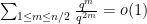
• (Prime number theorem for polynomials) A randomly selected monic polynomial of degree will be irreducible with probability when is fixed and is large.
• If is a random monic polynomial of degree , and is a random irreducible factor of (with each selected with probability ), then is approximately uniformly distributed in when is fixed and is large.
• The set of real numbers arising from the factorisation of a randomly selected polynomial of degree converges (in a suitable sense) to the Poisson-Dirichlet process when is fixed and is large.

The above list of facts addressed the large limit of the polynomial ring , where the order of the field is held fixed, but the degrees of the polynomials go to infinity. This is the limit that is most closely analogous to the integers . However, there is another interesting asymptotic limit of polynomial rings to consider, namely the large limit where it is now the degree that is held fixed, but the order of the field goes to infinity. Actually to simplify the exposition we will use the slightly more restrictive limit where the characteristic of the field goes to infinity (again keeping the degree fixed), although all of the results proven below for the large limit turn out to be true as well in the large limit.

The large (or large ) limit is technically a different limit than the large limit, but in practice the asymptotic statistics of the two limits often agree quite closely. For instance, here is the prime number theorem in the large limit:

Theorem 1 (Prime number theorem) The probability that a random monic polynomial of degree is irreducible is in the limit where is fixed and the characteristic goes to infinity.

Proof: There are monic polynomials of degree . If is irreducible, then the zeroes of are distinct and lie in the finite field , but do not lie in any proper subfield of that field. Conversely, every element of that does not lie in a proper subfield is the root of a unique monic polynomial in of degree (the minimal polynomial of ). Since the union of all the proper subfields of has size , the total number of irreducible polynomials of degree is thus , and the claim follows.

Remark 2 The above argument and inclusion-exclusion in fact gives the well known exact formula for the number of irreducible monic polynomials of degree .

Now we can give a precise connection between the cycle distribution of a random permutation, and (the large limit of) the irreducible factorisation of a polynomial, giving a (somewhat indirect, but still connected) link between permutation cycle decomposition and integer factorisation:

Theorem 3 The partition of a random monic polynomial of degree converges in distribution to the partition of a random permutation of length , in the limit where is fixed and the characteristic goes to infinity.

We can quickly prove this theorem as follows. We first need a basic fact:

Lemma 4 (Most polynomials square-free in large limit) A random monic polynomial of degree will be square-free with probability when is fixed and (or ) goes to infinity. In a similar spirit, two randomly selected monic polynomials of degree will be coprime with probability if are fixed and or goes to infinity.

Proof: For any polynomial of degree , the probability that is divisible by is at most . Summing over all polynomials of degree , and using the union bound, we see that the probability that is not squarefree is at most , giving the first claim. For the second, observe from the first claim (and the fact that has only a bounded number of factors) that is squarefree with probability , giving the claim.

Now we can prove the theorem. Elementary combinatorics tells us that the probability of a random permutation consisting of cycles of length for , where are nonnegative integers with , is precisely

since there are ways to write a given tuple of cycles in cycle notation in nondecreasing order of length, and ways to select the labels for the cycle notation. On the other hand, by Theorem 1 (and using Lemma 4 to isolate the small number of cases involving repeated factors) the number of monic polynomials of degree that are the product of irreducible polynomials of degree is

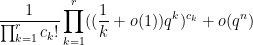
which simplifies to

and the claim follows.

This was a fairly short calculation, but it still doesn’t quite explain why there is such a link between the cycle decomposition of permutations and the factorisation of a polynomial. One immediate thought might be to try to link the multiplication structure of permutations in with the multiplication structure of polynomials; however, these structures are too dissimilar to set up a convincing analogy. For instance, the multiplication law on polynomials is abelian and non-invertible, whilst the multiplication law on is (extremely) non-abelian but invertible. Also, the multiplication of a degree and a degree polynomial is a degree polynomial, whereas the group multiplication law on permutations does not take a permutation in and a permutation in and return a permutation in .

I recently found (after some discussions with Ben Green) what I feel to be a satisfying conceptual (as opposed to computational) explanation of this link, which I will place below the fold.

Dwork’s proof of rationality of the zeta function over finite fields

Let be a quasiprojective variety defined over a finite field , thus for instance could be an affine variety

where is -dimensional affine space and are a finite collection of polynomials with coefficients in . Then one can define the set of -rational points, and more generally the set of -rational points for any , since can be viewed as a field extension of . Thus for instance in the affine case (1) we have

The Weil conjectures are concerned with understanding the number

of -rational points over a variety . The first of these conjectures was proven by Dwork, and can be phrased as follows.

Theorem 1 (Rationality of the zeta function) Let be a quasiprojective variety defined over a finite field , and let be given by (2). Then there exist a finite number of algebraic integers (known as characteristic values of ), such that

for all .

After cancelling, we may of course assume that for any and , and then it is easy to see (as we will see below) that the become uniquely determined up to permutations of the and . These values are known as the characteristic values of . Since is a rational integer (i.e. an element of ) rather than merely an algebraic integer (i.e. an element of the ring of integers of the algebraic closure of ), we conclude from the above-mentioned uniqueness that the set of characteristic values are invariant with respect to the Galois group . To emphasise this Galois invariance, we will not fix a specific embedding of the algebraic numbers into the complex field , but work with all such embeddings simultaneously. (Thus, for instance, contains three cube roots of , but which of these is assigned to the complex numbers , , will depend on the choice of embedding .)

An equivalent way of phrasing Dwork’s theorem is that the (-form of the) zeta function

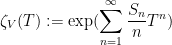
associated to (which is well defined as a formal power series in , at least) is equal to a rational function of (with the and being the poles and zeroes of respectively). Here, we use the formal exponential

Equivalently, the (-form of the) zeta-function is a meromorphic function on the complex numbers which is also periodic with period , and which has only finitely many poles and zeroes up to this periodicity.

Dwork’s argument relies primarily on -adic analysis – an analogue of complex analysis, but over an algebraically complete (and metrically complete) extension of the -adic field , rather than over the Archimedean complex numbers . The argument is quite effective, and in particular gives explicit upper bounds for the number of characteristic values in terms of the complexity of the variety ; for instance, in the affine case (1) with of degree , Bombieri used Dwork’s methods (in combination with Deligne’s theorem below) to obtain the bound , and a subsequent paper of Hooley established the slightly weaker bound purely from Dwork’s methods (a similar bound had also been pointed out in unpublished work of Dwork). In particular, one has bounds that are uniform in the field , which is an important fact for many analytic number theory applications.

These -adic arguments stand in contrast with Deligne’s resolution of the last (and deepest) of the Weil conjectures:

Theorem 2 (Riemann hypothesis) Let be a quasiprojective variety defined over a finite field , and let be a characteristic value of . Then there exists a natural number such that for every embedding , where denotes the usual absolute value on the complex numbers . (Informally: and all of its Galois conjugates have complex magnitude .)

To put it another way that closely resembles the classical Riemann hypothesis, all the zeroes and poles of the -form lie on the critical lines for . (See this previous blog post for further comparison of various instantiations of the Riemann hypothesis.) Whereas Dwork uses -adic analysis, Deligne uses the essentially orthogonal technique of ell-adic cohomology to establish his theorem. However, ell-adic methods can be used (via the Grothendieck-Lefschetz trace formula) to establish rationality, and conversely, in this paper of Kedlaya p-adic methods are used to establish the Riemann hypothesis. As pointed out by Kedlaya, the ell-adic methods are tied to the intrinsic geometry of (such as the structure of sheaves and covers over ), while the -adic methods are more tied to the extrinsic geometry of (how sits inside its ambient affine or projective space).

In this post, I would like to record my notes on Dwork’s proof of Theorem 1, drawing heavily on the expositions of Serre, Hooley, Koblitz, and others.

The basic strategy is to control the rational integers both in an “Archimedean” sense (embedding the rational integers inside the complex numbers with the usual norm ) as well as in the “-adic” sense, with the characteristic of (embedding the integers now in the “complexification” of the -adic numbers , which is equipped with a norm that we will recall later). (This is in contrast to the methods of ell-adic cohomology, in which one primarily works over an -adic field with .) The Archimedean control is trivial:

Proposition 3 (Archimedean control of ) With as above, and any embedding , we have

for all and some independent of .

Proof: Since is a rational integer, is just . By decomposing into affine pieces, we may assume that is of the affine form (1), then we trivially have , and the claim follows.

Another way of thinking about this Archimedean control is that it guarantees that the zeta function can be defined holomorphically on the open disk in of radius centred at the origin.

The -adic control is significantly more difficult, and is the main component of Dwork’s argument:

Proposition 4 (-adic control of ) With as above, and using an embedding (defined later) with the characteristic of , we can find for any real a finite number of elements such that

for all .

Another way of thinking about this -adic control is that it guarantees that the zeta function can be defined meromorphically on the entire -adic complex field .

Proposition 4 is ostensibly much weaker than Theorem 1 because of (a) the error term of -adic magnitude at most ; (b) the fact that the number of potential characteristic values here may go to infinity as ; and (c) the potential characteristic values only exist inside the complexified -adics , rather than in the algebraic integers . However, it turns out that by combining -adic control on in Proposition 4 with the trivial control on in Proposition 3, one can obtain Theorem 1 by an elementary argument that does not use any further properties of (other than the obvious fact that the are rational integers), with the in Proposition 4 chosen to exceed the in Proposition 3. We give this argument (essentially due to Borel) below the fold.

The proof of Proposition 4 can be split into two pieces. The first piece, which can be viewed as the number-theoretic component of the proof, uses external descriptions of such as (1) to obtain the following decomposition of :

Proposition 5 (Decomposition of ) With and as above, we can decompose as a finite linear combination (over the integers) of sequences , such that for each such sequence , the zeta functions

are entire in , by which we mean that

as .

This proposition will ultimately be a consequence of the properties of the Teichmuller lifting .

The second piece, which can be viewed as the “-adic complex analytic” component of the proof, relates the -adic entire nature of a zeta function with control on the associated sequence , and can be interpreted (after some manipulation) as a -adic version of the Weierstrass preparation theorem:

Proposition 6 (-adic Weierstrass preparation theorem) Let be a sequence in , such that the zeta function

is entire in . Then for any real , there exist a finite number of elements such that

for all and some .

Clearly, the combination of Proposition 5 and Proposition 6 (and the non-Archimedean nature of the norm) imply Proposition 4.

The Bombieri-Stepanov proof of the Hasse-Weil bound

Let be a finite field of order , and let be an absolutely irreducible smooth projective curve defined over (and hence over the algebraic closure of that field). For instance, could be the projective elliptic curve

in the projective plane , where are coefficients whose discriminant is non-vanishing, which is the projective version of the affine elliptic curve

To each such curve one can associate a genus , which we will define later; for instance, elliptic curves have genus . We can also count the cardinality of the set of -points of . The Hasse-Weil bound relates the two:

Theorem 1 (Hasse-Weil bound) .

The usual proofs of this bound proceed by first establishing a trace formula of the form

 

for some complex numbers independent of ; this is in fact a special case of the Lefschetz-Grothendieck trace formula, and can be interpreted as an assertion that the zeta function associated to the curve is rational. The task is then to establish a bound for all ; this (or more precisely, the slightly stronger assertion ) is the Riemann hypothesis for such curves. This can be done either by passing to the Jacobian variety of and using a certain duality available on the cohomology of such varieties, known as Rosati involution; alternatively, one can pass to the product surface and apply the Riemann-Roch theorem for that surface.

In 1969, Stepanov introduced an elementary method (a version of what is now known as the polynomial method) to count (or at least to upper bound) the quantity . The method was initially restricted to hyperelliptic curves, but was soon extended to general curves. In particular, Bombieri used this method to give a short proof of the following weaker version of the Hasse-Weil bound:

Theorem 2 (Weak Hasse-Weil bound) If is a perfect square, and , then .

In fact, the bound on can be sharpened a little bit further, as we will soon see.

Theorem 2 is only an upper bound on , but there is a Galois-theoretic trick to convert (a slight generalisation of) this upper bound to a matching lower bound, and if one then uses the trace formula (1) (and the “tensor power trick” of sending to infinity to control the weights ) one can then recover the full Hasse-Weil bound. We discuss these steps below the fold.

I’ve discussed Bombieri’s proof of Theorem 2 in this previous post (in the special case of hyperelliptic curves), but now wish to present the full proof, with some minor simplifications from Bombieri’s original presentation; it is mostly elementary, with the deepest fact from algebraic geometry needed being Riemann’s inequality (a weak form of the Riemann-Roch theorem).

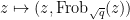
The first step is to reinterpret as the number of points of intersection between two curves in the surface . Indeed, if we define the Frobenius endomorphism on any projective space by

then this map preserves the curve , and the fixed points of this map are precisely the points of :

Thus one can interpret as the number of points of intersection between the diagonal curve

and the Frobenius graph

which are copies of inside . But we can use the additional hypothesis that is a perfect square to write this more symmetrically, by taking advantage of the fact that the Frobenius map has a square root

with also preserving . One can then also interpret as the number of points of intersection between the curve

 

and its transpose

Let be the field of rational functions on (with coefficients in ), and define , , and analogously )(although is likely to be disconnected, so will just be a ring rather than a field. We then (morally) have the commuting square

if we ignore the issue that a rational function on, say, , might blow up on all of and thus not have a well-defined restriction to . We use and to denote the restriction maps. Furthermore, we have obvious isomorphisms , coming from composing with the graphing maps and .

The idea now is to find a rational function on the surface of controlled degree which vanishes when restricted to , but is non-vanishing (and not blowing up) when restricted to . On , we thus get a non-zero rational function of controlled degree which vanishes on – which then lets us bound the cardinality of in terms of the degree of . (In Bombieri’s original argument, one required vanishing to high order on the side, but in our presentation, we have factored out a term which removes this high order vanishing condition.)

To find this , we will use linear algebra. Namely, we will locate a finite-dimensional subspace of (consisting of certain “controlled degree” rational functions) which projects injectively to , but whose projection to has strictly smaller dimension than itself. The rank-nullity theorem then forces the existence of a non-zero element of whose projection to vanishes, but whose projection to is non-zero.

Now we build . Pick a point of , which we will think of as being a point at infinity. (For the purposes of proving Theorem 2, we may clearly assume that is non-empty.) Thus is fixed by . To simplify the exposition, we will also assume that is fixed by the square root of ; in the opposite case when has order two when acting on , the argument is essentially the same, but all references to in the second factor of need to be replaced by (we leave the details to the interested reader).

For any natural number , define to be the set of rational functions which are allowed to have a pole of order up to at , but have no other poles on ; note that as we are assuming to be smooth, it is unambiguous what a pole is (and what order it will have). (In the fancier language of divisors and Cech cohomology, we have .) The space is clearly a vector space over ; one can view intuitively as the space of “polynomials” on of “degree” at most . When , consists just of the constant functions. Indeed, if , then the image of avoids and so lies in the affine line ; but as is projective, the image needs to be compact (hence closed) in , and must therefore be a point, giving the claim.

For higher , we have the easy relations

 

The former inequality just comes from the trivial inclusion . For the latter, observe that if two functions lie in , so that they each have a pole of order at most at , then some linear combination of these functions must have a pole of order at most at ; thus has codimension at most one in , giving the claim.

From (3) and induction we see that each of the are finite dimensional, with the trivial upper bound

 

Riemann’s inequality complements this with the lower bound

 

thus one has for all but at most exceptions (in fact, exactly exceptions as it turns out). This is a consequence of the Riemann-Roch theorem; it can be proven from abstract nonsense (the snake lemma) if one defines the genus in a non-standard fashion (as the dimension of the first Cech cohomology of the structure sheaf of ), but to obtain this inequality with a standard definition of (e.g. as the dimension of the zeroth Cech cohomolgy of the line bundle of differentials) requires the more non-trivial tool of Serre duality.

At any rate, now that we have these vector spaces , we will define to be a tensor product space

for some natural numbers which we will optimise in later. That is to say, is spanned by functions of the form with and . This is clearly a linear subspace of of dimension , and hence by Rieman’s inequality we have

 

if

 

Observe that maps a tensor product to a function . If and , then we see that the function has a pole of order at most at . We conclude that

 

and in particular by (4)

 

and similarly

 

We will choose to be a bit bigger than , to make the image of smaller than that of . From (6), (10) we see that if we have the inequality

 

(together with (7)) then cannot be injective.

On the other hand, we have the following basic fact:

Lemma 3 (Injectivity) If

 

then is injective.

Proof: From (3), we can find a linear basis of such that each of the has a distinct order of pole at (somewhere between and inclusive). Similarly, we may find a linear basis of such that each of the has a distinct order of pole at (somewhere between and inclusive). The functions then span , and the order of pole at is . But since , these orders are all distinct, and so these functions must be linearly independent. The claim follows.

This gives us the following bound:

Proposition 4 Let be natural numbers such that (7), (11), (12) hold. Then .

Proof: As is not injective, we can find with vanishing. By the above lemma, the function is then non-zero, but it must also vanish on , which has cardinality . On the other hand, by (8), has a pole of order at most at and no other poles. Since the number of poles and zeroes of a rational function on a projective curve must add up to zero, the claim follows.

If , we may make the explicit choice

and a brief calculation then gives Theorem 2. In some cases one can optimise things a bit further. For instance, in the genus zero case (e.g. if is just the projective line ) one may take and conclude the absolutely sharp bound in this case; in the case of the projective line , the function is in fact the very concrete function .

Remark 1 When is not a perfect square, one can try to run the above argument using the factorisation instead of . This gives a weaker version of the above bound, of the shape . In the hyperelliptic case at least, one can erase this loss by working with a variant of the argument in which one requires to vanish to high order at , rather than just to first order; see this survey article of mine for details.

Multiple recurrence and convergence results associated to F_p^omega-actions

Vitaly Bergelson, Tamar Ziegler, and I have just uploaded to the arXiv our joint paper “Multiple recurrence and convergence results associated to -actions“. This paper is primarily concerned with limit formulae in the theory of multiple recurrence in ergodic theory. Perhaps the most basic formula of this type is the mean ergodic theorem, which (among other things) asserts that if is a measure-preserving -system (which, in this post, means that is a probability space and is measure-preserving and invertible, thus giving an action of the integers), and are functions, and is ergodic (which means that contains no -invariant functions other than the constants (up to almost everywhere equivalence, of course)), then the average

converges as to the expression

see e.g. this previous blog post. Informally, one can interpret this limit formula as an equidistribution result: if is drawn at random from (using the probability measure ), and is drawn at random from for some large , then the pair becomes uniformly distributed in the product space (using product measure ) in the limit as .

If we allow to be non-ergodic, then we still have a limit formula, but it is a bit more complicated. Let be the -invariant measurable sets in ; the -system can then be viewed as a factor of the original system , which is equivalent (in the sense of measure-preserving systems) to a trivial system (known as the invariant factor) in which the shift is trivial. There is then a projection map to the invariant factor which is a factor map, and the average (1) converges in the limit to the expression

where is the pushforward map associated to the map ; see e.g. this previous blog post. We can interpret this as an equidistribution result. If is a pair as before, then we no longer expect complete equidistribution in in the non-ergodic, because there are now non-trivial constraints relating with ; indeed, for any -invariant function , we have the constraint ; putting all these constraints together we see that (for almost every , at least). The limit (2) can be viewed as an assertion that this constraint are in some sense the “only” constraints between and , and that the pair is uniformly distributed relative to these constraints.

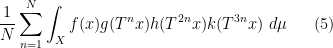
Limit formulae are known for multiple ergodic averages as well, although the statement becomes more complicated. For instance, consider the expression

for three functions ; this is analogous to the combinatorial task of counting length three progressions in various sets. For simplicity we assume the system to be ergodic. Naively one might expect this limit to then converge to

which would roughly speaking correspond to an assertion that the triplet is asymptotically equidistributed in . However, even in the ergodic case there can be additional constraints on this triplet that cannot be seen at the level of the individual pairs , . The key obstruction here is that of eigenfunctions of the shift , that is to say non-trivial functions that obey the eigenfunction equation almost everywhere for some constant (or -invariant) . Each such eigenfunction generates a constraint

tying together , , and . However, it turns out that these are in some sense the only constraints on that are relevant for the limit (3). More precisely, if one sets to be the sub-algebra of generated by the eigenfunctions of , then it turns out that the factor is isomorphic to a shift system known as the Kronecker factor, for some compact abelian group and some (irrational) shift ; the factor map pushes eigenfunctions forward to (affine) characters on . It is then known that the limit of (3) is

where is the closed subgroup

and is the Haar probability measure on ; see this previous blog post. The equation defining corresponds to the constraint (4) mentioned earlier. Among other things, this limit formula implies Roth’s theorem, which in the context of ergodic theory is the assertion that the limit (or at least the limit inferior) of (3) is positive when is non-negative and not identically vanishing.

If one considers a quadruple average

(analogous to counting length four progressions) then the situation becomes more complicated still, even in the ergodic case. In addition to the (linear) eigenfunctions that already showed up in the computation of the triple average (3), a new type of constraint also arises from quadratic eigenfunctions , which obey an eigenfunction equation in which is no longer constant, but is now a linear eigenfunction. For such functions, behaves quadratically in , and one can compute the existence of a constraint

between , , , and that is not detected at the triple average level. As it turns out, this is not the only type of constraint relevant for (5); there is a more general class of constraint involving two-step nilsystems which we will not detail here, but see e.g. this previous blog post for more discussion. Nevertheless there is still a similar limit formula to previous examples, involving a special factor which turns out to be an inverse limit of two-step nilsystems; this limit theorem can be extracted from the structural theory in this paper of Host and Kra combined with a limit formula for nilsystems obtained by Lesigne, but will not be reproduced here. The pattern continues to higher averages (and higher step nilsystems); this was first done explicitly by Ziegler, and can also in principle be extracted from the structural theory of Host-Kra combined with nilsystem equidistribution results of Leibman. These sorts of limit formulae can lead to various recurrence results refining Roth’s theorem in various ways; see this paper of Bergelson, Host, and Kra for some examples of this.

The above discussion was concerned with -systems, but one can adapt much of the theory to measure-preserving -systems for other discrete countable abelian groups , in which one now has a family of shifts indexed by rather than a single shift, obeying the compatibility relation . The role of the intervals in this more general setting is replaced by that of Folner sequences. For arbitrary countable abelian , the theory for double averages (1) and triple limits (3) is essentially identical to the -system case. But when one turns to quadruple and higher limits, the situation becomes more complicated (and, for arbitrary , still not fully understood). However one model case which is now well understood is the finite field case when is an infinite-dimensional vector space over a finite field (with the finite subspaces then being a good choice for the Folner sequence). Here, the analogue of the structural theory of Host and Kra was worked out by Vitaly, Tamar, and myself in these previous papers (treating the high characteristic and low characteristic cases respectively). In the finite field setting, it turns out that nilsystems no longer appear, and one only needs to deal with linear, quadratic, and higher order eigenfunctions (known collectively as phase polynomials). It is then natural to look for a limit formula that asserts, roughly speaking, that if is drawn at random from a -system and drawn randomly from a large subspace of , then the only constraints between are those that arise from phase polynomials. The main theorem of this paper is to establish this limit formula (which, again, is a little complicated to state explicitly and will not be done here). In particular, we establish for the first time that the limit actually exists (a result which, for -systems, was one of the main results of this paper of Host and Kra).

As a consequence, we can recover finite field analogues of most of the results of Bergelson-Host-Kra, though interestingly some of the counterexamples demonstrating sharpness of their results for -systems (based on Behrend set constructions) do not seem to be present in the finite field setting (cf. this previous blog post on the cap set problem). In particular, we are able to largely settle the question of when one has a Khintchine-type theorem that asserts that for any measurable set in an ergodic -system and any , one has

for a syndetic set of , where are distinct residue classes. It turns out that Khintchine-type theorems always hold for (and for ergodicity is not required), and for it holds whenever form a parallelogram, but not otherwise (though the counterexample here was such a painful computation that we ended up removing it from the paper, and may end up putting it online somewhere instead), and for larger we could show that the Khintchine property failed for generic choices of , though the problem of determining exactly the tuples for which the Khintchine property failed looked to be rather messy and we did not completely settle it.

Definable subsets over (nonstandard) finite fields, and almost quantifier elimination

Much as group theory is the study of groups, or graph theory is the study of graphs, model theory is the study of models (also known as structures) of some language (which, in this post, will always be a single-sorted, first-order language). A structure is a set , equipped with one or more operations, constants, and relations. This is of course an extremely general type of mathematical object, but (quite remarkably) one can still say a substantial number of interesting things about very broad classes of structures.

We will observe the common abuse of notation of using the set as a metonym for the entire structure, much as we usually refer to a group simply as , a vector space simply as , and so forth. Following another common bending of the rules, we also allow some operations on structures (such as the multiplicative inverse operation on a group or field) to only be partially defined, and we allow use of the usual simplifying conventions for mathematical formulas (e.g. writing instead of or , in cases where associativity is known). We will also deviate slightly from the usual practice in logic by emphasising individual structures, rather than the theory of general classes of structures; for instance, we will talk about the theory of a single field such as or , rather than the theory of all fields of a certain type (e.g. real closed fields or algebraically closed fields).

Once one has a structure , one can introduce the notion of a definable subset of , or more generally of a Cartesian power of , defined as a set of the form

for some formula in the language with free variables and any number of constants from (that is, is a well-formed formula built up from a finite number of constants in , the relations and operations on , logical connectives such as , , , and the quantifiers ). Thus, for instance, in the theory of the arithmetic of the natural numbers , the set of primes is a definable set, since we have

In the theory of the field of reals , the unit circle is an example of a definable set,

but so is the the complement of the circle,

and the interval :

Due to the unlimited use of constants, any finite subset of a power of any structure is, by our conventions, definable in that structure. (One can of course also consider definability without parameters (also known as -definability), in which arbitrary constants are not permitted, but we will not do so here.)

We can isolate some special subclasses of definable sets:

• An atomic definable set is a set of the form (1) in which is an atomic formula (i.e. it does not contain any logical connectives or quantifiers).
• A quantifier-free definable set is a set of the form (1) in which is quantifier-free (i.e. it can contain logical connectives, but does not contain the quantifiers ).

Example 1 In the theory of a field such as , an atomic definable set is the same thing as an affine algebraic set (also known as an affine algebraic variety, with the understanding that varieties are not necessarily assumed to be irreducible), and a quantifier-free definable set is known as a constructible set; thus we see that algebraic geometry can be viewed in some sense as a special case of model theory. (Conversely, it can in fact be quite profitable to think of model theory as an abstraction of algebraic geometry; for instance, the concepts of Morley rank and Morley degree in model theory (discussed in this previous blog post) directly generalises the concepts of dimension and degree in algebraic geometry.) Over , the interval is a definable set, but not a quantifier-free definable set (and certainly not an atomic definable set); and similarly for the primes over .

A quantifier-free definable set in is nothing more than a finite boolean combination of atomic definable sets; in other words, the class of quantifier-free definable sets over is the smallest class that contains the atomic definable sets and is closed under boolean operations such as complementation and union (which generate all the other boolean operations). Similarly, the class of definable sets over is the smallest class that contains the quantifier-free definable sets, and is also closed under the operation of projection from to for every natural number , where is the map .

Some structures have the property of enjoying quantifier elimination, which means that every definable set is in fact a quantifier-free definable set, or equivalently that the projection of a quantifier-free definable set is again quantifier-free. For instance, an algebraically closed field (with the field operations) has quantifier elimination (i.e. the projection of a constructible set is again constructible); this fact can be proven by the classical tool of resultants, and among other things can be used to give a proof of Hilbert’s nullstellensatz. (Note though that projection does not necessary preserve the property of being atomic; for instance, the projection of the atomic set is the non-atomic, but still quantifier-free definable, set .) In the converse direction, it is not difficult to use the nullstellensatz to deduce quantifier elimination. For theory of the real field , which is not algebraically closed, one does not have quantifier elimination, as one can see from the example of the unit circle (which is a quantifier-free definable set) projecting down to the interval (which is definable, but not quantifer-free definable). However, if one adds the additional operation of order to the reals, giving it the language of an ordered field rather than just a field, then quantifier elimination is recovered (the class of quantifier-free definable sets now enlarges to match the class of definable sets, which in this case is also the class of semi-algebraic sets); this is the famous Tarski-Seidenberg theorem.

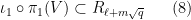
On the other hand, many important structures do not have quantifier elimination; typically, the projection of a quantifier-free definable set is not, in general, quantifier-free definable. This failure of the projection property also shows up in many contexts outside of model theory; for instance, Lebesgue famously made the error of thinking that the projection of a Borel measurable set remained Borel measurable (it is merely an analytic set instead). Turing’s halting theorem can be viewed as an assertion that the projection of a decidable set (also known as a computable or recursive set) is not necessarily decidable (it is merely semi-decidable (or recursively enumerable) instead). The notorious P=NP problem can also be essentially viewed in this spirit; roughly speaking (and glossing over the placement of some quantifiers), it asks whether the projection of a polynomial-time decidable set is again polynomial-time decidable. And so forth. (See this blog post of Dick Lipton for further discussion of the subtleties of projections.)

Now we consider the status of quantifier elimination for the theory of a finite field . If interpreted naively, quantifier elimination is trivial for a finite field , since every subset of is finite and thus quantifier-free definable. However, we can recover an interesting question in one of two (essentially equivalent) ways. One is to work in the asymptotic regime in which the field is large, but the length of the formulae used to construct one’s definable sets stays bounded uniformly in the size of (where we view any constant in as contributing a unit amount to the length of a formula, no matter how large is). A simple counting argument then shows that only a small number of subsets of become definable in the asymptotic limit , since the number of definable sets clearly grows at most polynomially in for any fixed bound on the formula length, while the number of all subsets of grows exponentially in .

Another way to proceed is to work not with a single finite field , or even with a sequence of finite fields, but with the ultraproduct of a sequence of finite fields, and to study the properties of definable sets over this ultraproduct. (We will be using the notation of ultraproducts and nonstandard analysis from this previous blog post.) This approach is equivalent to the more finitary approach mentioned in the previous paragraph, at least if one does not care to track of the exact bounds on the length of the formulae involved. Indeed, thanks to Los’s theorem, a definable subset of is nothing more than the ultraproduct of definable subsets of for all sufficiently close to , with the length of the formulae used to define uniformly bounded in . In the language of nonstandard analysis, one can view as a nonstandard finite field.

The ultraproduct of finite fields is an important example of a pseudo-finite field – a field that obeys all the sentences in the languages of fields that finite fields do, but is not necessarily itself a finite field. The model theory of pseudo-finite fields was first studied systematically by Ax (in the same paper where the Ax-Grothendieck theorem, discussed previously on this blog, was established), with important further contributions by Kiefe, by Fried-Sacerdote, by two papers of Chatzidakis-van den Dries-Macintyre, and many other authors.

As mentioned before, quantifier elimination trivially holds for finite fields. But for infinite pseudo-finite fields, such as the ultraproduct of finite fields with going to infinity, quantifier elimination fails. For instance, in a finite field , the set of quadratic residues is a definable set, with a bounded formula length, and so in the ultraproduct , the set of nonstandard quadratic residues is also a definable set. However, in one dimension, we see from the factor theorem that the only atomic definable sets are either finite or the whole field , and so the only constructible sets (i.e. the only quantifier-free definable sets) are either finite or cofinite in . Since the quadratic residues have asymptotic density in a large finite field, they cannot form a quantifier-free definable set, despite being definable.

Nevertheless, there is a very nice almost quantifier elimination result for these fields, in characteristic zero at least, which we phrase here as follows:

Theorem 1 (Almost quantifier elimination) Let be a nonstandard finite field of characteristic zero, and let be a definable set over . Then is the union of finitely many sets of the form

where is an atomic definable subset of (i.e. the -points of an algebraic variety defined over in ) and is a polynomial.

Results of this type were first obtained essentially due to Catarina Kiefe, although the formulation here is closer to that of Chatzidakis-van den Dries-Macintyre.

Informally, this theorem says that while we cannot quite eliminate all quantifiers from a definable set over a nonstandard finite field, we can eliminate all but one existential quantifier. Note that negation has also been eliminated in this theorem; for instance, the definable set uses a negation, but can also be described using a single existential quantifier as .) I believe that there are more complicated analogues of this result in positive characteristic, but I have not studied this case in detail (Kiefe’s result does not assume characteristic zero, but her conclusion is slightly different from the one given here). In the one-dimensional case , the only varieties are the affine line and finite sets, and we can simplify the above statement, namely that any definable subset of takes the form for some polynomial (i.e. definable sets in are nothing more than the projections of the -points of a plane curve).

There is an equivalent formulation of this theorem for standard finite fields, namely that if is a finite field and is definable using a formula of length at most , then can be expressed in the form (2) with the degree of bounded by some quantity depending on and , assuming that the characteristic of is sufficiently large depending on .

The theorem gives quite a satisfactory description of definable sets in either standard or nonstandard finite fields (at least if one does not care about effective bounds in some of the constants, and if one is willing to exclude the small characteristic case); for instance, in conjunction with the Lang-Weil bound discussed in this recent blog post, it shows that any non-empty definable subset of a nonstandard finite field has a nonstandard cardinality of for some positive standard rational and integer . Equivalently, any non-empty definable subset of for some standard finite field using a formula of length at most has a standard cardinality of for some positive rational of height and some natural number between and . (For instance, in the example of the quadratic residues given above, is equal to and equal to .) There is a more precise statement to this effect, namely that the Poincaré series of a definable set is rational; see Kiefe’s paper for details.

Below the fold I give a proof of Theorem 1, which relies primarily on the Lang-Weil bound mentioned above.

The Lang-Weil bound

Let be a finite field, with algebraic closure , and let be an (affine) algebraic variety defined over , by which I mean a set of the form

for some ambient dimension , and some finite number of polynomials . In order to reduce the number of subscripts later on, let us say that has complexity at most if , , and the degrees of the are all less than or equal to . Note that we do not require at this stage that be irreducible (i.e. not the union of two strictly smaller varieties), or defined over , though we will often specialise to these cases later in this post. (Also, everything said here can also be applied with almost no changes to projective varieties, but we will stick with affine varieties for sake of concreteness.)

One can consider two crude measures of how “big” the variety is. The first measure, which is algebraic geometric in nature, is the dimension of the variety , which is an integer between and (or, depending on convention, , , or undefined, if is empty) that can be defined in a large number of ways (e.g. it is the largest for which the generic linear projection from to is dominant, or the smallest for which the intersection with a generic codimension subspace is non-empty). The second measure, which is number-theoretic in nature, is the number of -points of , i.e. points in all of whose coefficients lie in the finite field, or equivalently the number of solutions to the system of equations for with variables in .

These two measures are linked together in a number of ways. For instance, we have the basic Schwarz-Zippel type bound (which, in this qualitative form, goes back at least to Lemma 1 of the work of Lang and Weil in 1954).

Lemma 1 (Schwarz-Zippel type bound) Let be a variety of complexity at most . Then we have .

Proof: (Sketch) For the purposes of exposition, we will not carefully track the dependencies of implied constants on the complexity , instead simply assuming that all of these quantities remain controlled throughout the argument. (If one wished, one could obtain ineffective bounds on these quantities by an ultralimit argument, as discussed in this previous post, or equivalently by moving everything over to a nonstandard analysis framework; one could also obtain such uniformity using the machinery of schemes.)

We argue by induction on the ambient dimension of the variety . The case is trivial, so suppose and that the claim has already been proven for . By breaking up into irreducible components we may assume that is irreducible (this requires some control on the number and complexity of these components, but this is available, as discussed in this previous post). For each , the fibre is either one-dimensional (and thus all of ) or zero-dimensional. In the latter case, one has points in the fibre from the fundamental theorem of algebra (indeed one has a bound of in this case), and lives in the projection of to , which is a variety of dimension at most and controlled complexity, so the contribution of this case is acceptable from the induction hypothesis. In the former case, the fibre contributes -points, but lies in a variety in of dimension at most (since otherwise would contain a subvariety of dimension at least , which is absurd) and controlled complexity, and so the contribution of this case is also acceptable from the induction hypothesis.

One can improve the bound on the implied constant to be linear in the degree of (see e.g. Claim 7.2 of this paper of Dvir, Kollar, and Lovett, or Lemma A.3 of this paper of Ellenberg, Oberlin, and myself), but we will not be concerned with these improvements here.

Without further hypotheses on , the above upper bound is sharp (except for improvements in the implied constants). For instance, the variety

where are distict, is the union of distinct hyperplanes of dimension , with and complexity ; similar examples can easily be concocted for other choices of . In the other direction, there is also no non-trivial lower bound for without further hypotheses on . For a trivial example, if is an element of that does not lie in , then the hyperplane

clearly has no -points whatsoever, despite being a -dimensional variety in of complexity . For a slightly less non-trivial example, if is an element of that is not a quadratic residue, then the variety

which is the union of two hyperplanes, still has no -points, even though this time the variety is defined over instead of (by which we mean that the defining polynomial(s) have all of their coefficients in ). There is however the important Lang-Weil bound that allows for a much better estimate as long as is both defined over and irreducible:

Theorem 2 (Lang-Weil bound) Let be a variety of complexity at most . Assume that is defined over , and that is irreducible as a variety over (i.e. is geometrically irreducible or absolutely irreducible). Then

Again, more explicit bounds on the implied constant here are known, but will not be the focus of this post. As the previous examples show, the hypotheses of definability over and geometric irreducibility are both necessary.

The Lang-Weil bound is already non-trivial in the model case of plane curves:

Theorem 3 (Hasse-Weil bound) Let be an irreducible polynomial of degree with coefficients in . Then

Thus, for instance, if , then the elliptic curve has -points, a result first established by Hasse. The Hasse-Weil bound is already quite non-trivial, being the analogue of the Riemann hypothesis for plane curves. For hyper-elliptic curves, an elementary proof (due to Stepanov) is discussed in this previous post. For general plane curves, the first proof was by Weil (leading to his famous Weil conjectures); there is also a nice version of Stepanov’s argument due to Bombieri covering this case which is a little less elementary (relying crucially on the Riemann-Roch theorem for the upper bound, and a lifting trick to then get the lower bound), which I briefly summarise later in this post. The full Lang-Weil bound is deduced from the Hasse-Weil bound by an induction argument using generic hyperplane slicing, as I will also summarise later in this post.

The hypotheses of definability over and geometric irreducibility in the Lang-Weil can be removed after inserting a geometric factor:

Corollary 4 (Lang-Weil bound, alternate form) Let be a variety of complexity at most . Then one has

where is the number of top-dimensional components of (i.e. geometrically irreducible components of of dimension ) that are definable over , or equivalently are invariant with respect to the Frobenius endomorphism that defines .

Proof: By breaking up a general variety into components (and using Lemma 1 to dispose of any lower-dimensional components), it suffices to establish this claim when is itself geometrically irreducible. If is definable over , the claim follows from Theorem 2. If is not definable over , then it is not fixed by the Frobenius endomorphism (since otherwise one could produce a set of defining polynomials that were fixed by Frobenius and thus defined over by using some canonical basis (such as a reduced Grobner basis) for the associated ideal), and so has strictly smaller dimension than . But captures all the -points of , so in this case the claim follows from Lemma 1.

Note that if is reducible but is itself defined over , then the Frobenius endomorphism preserves itself, but may permute the components of around. In this case, is the number of fixed points of this permutation action of Frobenius on the components. In particular, is always a natural number between and ; thus we see that regardless of the geometry of , the normalised count is asymptotically restricted to a bounded range of natural numbers (in the regime where the complexity stays bounded and goes to infinity).

Example 1 Consider the variety

for some non-zero parameter . Geometrically (by which we basically mean “when viewed over the algebraically closed field “), this is the union of two lines, with slopes corresponding to the two square roots of . If is a quadratic residue, then both of these lines are defined over , and are fixed by Frobenius, and in this case. If is not a quadratic residue, then the lines are not defined over , and the Frobenius automorphism permutes the two lines while preserving as a whole, giving in this case.

Corollary 4 effectively computes (at least to leading order) the number-theoretic size of a variety in terms of geometric information about , namely its dimension and the number of top-dimensional components fixed by Frobenius. It turns out that with a little bit more effort, one can extend this connection to cover not just a single variety , but a family of varieties indexed by points in some base space . More precisely, suppose we now have two affine varieties of bounded complexity, together with a regular map of bounded complexity (the definition of complexity of a regular map is a bit technical, see e.g. this paper, but one can think for instance of a polynomial or rational map of bounded degree as a good example). It will be convenient to assume that the base space is irreducible. If the map is a dominant map (i.e. the image is Zariski dense in ), then standard algebraic geometry results tell us that the fibres are an unramified family of -dimensional varieties outside of an exceptional subset of of dimension strictly smaller than (and with having dimension strictly smaller than ); see e.g. Section I.6.3 of Shafarevich.

Now suppose that , , and are defined over . Then, by Lang-Weil, has -points, and by Schwarz-Zippel, for all but of these -points (the ones that lie in the subvariety ), the fibre is an algebraic variety defined over of dimension . By using ultraproduct arguments (see e.g. Lemma 3.7 of this paper of mine with Emmanuel Breuillard and Ben Green), this variety can be shown to have bounded complexity, and thus by Corollary 4, has -points. One can then ask how the quantity is distributed. A simple but illustrative example occurs when and is the polynomial . Then equals when is a non-zero quadratic residue and when is a non-zero quadratic non-residue (and when is zero, but this is a negligible fraction of all ). In particular, in the asymptotic limit , is equal to half of the time and half of the time.

Now we describe the asymptotic distribution of the . We need some additional notation. Let be an -point in , and let be the connected components of the fibre . As is defined over , this set of components is permuted by the Frobenius endomorphism . But there is also an action by monodromy of the fundamental group (this requires a certain amount of étale machinery to properly set up, as we are working over a positive characteristic field rather than over the complex numbers, but I am going to ignore this rather important detail here, as I still don’t fully understand it). This fundamental group may be infinite, but (by the étale construction) is always profinite, and in particular has a Haar probability measure, in which every finite index subgroup (and their cosets) are measurable. Thus we may meaningfully talk about elements drawn uniformly at random from this group, so long as we work only with the profinite -algebra on that is generated by the cosets of the finite index subgroups of this group (which will be the only relevant sets we need to measure when considering the action of this group on finite sets, such as the components of a generic fibre).

Theorem 5 (Lang-Weil with parameters) Let be varieties of complexity at most with irreducible, and let be a dominant map of complexity at most . Let be an -point of . Then, for any natural number , one has for values of , where is the random variable that counts the number of components of a generic fibre that are invariant under , where is an element chosen uniformly at random from the étale fundamental group . In particular, in the asymptotic limit , and with chosen uniformly at random from , (or, equivalently, ) and have the same asymptotic distribution.

This theorem generalises Corollary 4 (which is the case when is just a point, so that is just and is trivial). Informally, the effect of a non-trivial parameter space on the Lang-Weil bound is to push around the Frobenius map by monodromy for the purposes of counting invariant components, and a randomly chosen set of parameters corresponds to a randomly chosen loop on which to perform monodromy.

Example 2 Let and for some fixed ; to avoid some technical issues let us suppose that is coprime to . Then can be taken to be , and for a base point we can take . The fibre – the roots of unity – can be identified with the cyclic group by using a primitive root of unity. The étale fundamental group is (I think) isomorphic to the profinite closure of the integers (excluding the part of that closure coming from the characteristic of ). Not coincidentally, the integers are the fundamental group of the complex analogue of . (Brian Conrad points out to me though that for more complicated varieties, such as covers of by a power of the characteristic, the etale fundamental group is more complicated than just a profinite closure of the ordinary fundamental group, due to the presence of Artin-Schreier covers that are only ramified at infinity.) The action of this fundamental group on the fibres can given by translation. Meanwhile, the Frobenius map on is given by multiplication by . A random element then becomes a random affine map on , where chosen uniformly at random from . The number of fixed points of this map is equal to the greatest common divisor of and when is divisible by , and equal to otherwise. This matches up with the elementary number fact that a randomly chosen non-zero element of will be an power with probability , and when this occurs, the number of roots in will be .

Example 3 (Thanks to Jordan Ellenberg for this example.) Consider a random elliptic curve , where are chosen uniformly at random, and let . Let be the -torsion points of (i.e. those elements with using the elliptic curve addition law); as a group, this is isomorphic to (assuming that has sufficiently large characteristic, for simplicity), and consider the number of points of , which is a random variable taking values in the natural numbers between and . In this case, the base variety is the modular curve , and the covering variety is the modular curve . The generic fibre here can be identified with , the monodromy action projects down to the action of , and the action of Frobenius on this fibre can be shown to be given by a matrix with determinant (with the exact choice of matrix depending on the choice of fibre and of the identification), so the distribution of the number of -points of is asymptotic to the distribution of the number of fixed points of a random linear map of determinant on .

Theorem 5 seems to be well known “folklore” among arithmetic geometers, though I do not know of an explicit reference for it. I enjoyed deriving it for myself (though my derivation is somewhat incomplete due to my lack of understanding of étale cohomology) from the ordinary Lang-Weil theorem and the moment method. I’m recording this derivation later in this post, mostly for my own benefit (as I am still in the process of learning this material), though perhaps some other readers may also be interested in it.

Caveat: not all details are fully fleshed out in this writeup, particularly those involving the finer points of algebraic geometry and étale cohomology, as my understanding of these topics is not as complete as I would like it to be.

Many thanks to Brian Conrad and Jordan Ellenberg for helpful discussions on these topics.

New bounds for Szemeredi’s theorem, Ia: Progressions of length 4 in finite field geometries revisited

Ben Green and I have just uploaded to the arXiv our paper “New bounds for Szemeredi’s theorem, Ia: Progressions of length 4 in finite field geometries revisited“, submitted to Proc. Lond. Math. Soc.. This is both an erratum to, and a replacement for, our previous paper “New bounds for Szemeredi’s theorem. I. Progressions of length 4 in finite field geometries“. The main objective in both papers is to bound the quantity for a vector space over a finite field of characteristic greater than , where is defined as the cardinality of the largest subset of that does not contain an arithmetic progression of length . In our earlier paper, we gave two arguments that bounded in the regime when the field was fixed and was large. The first “cheap” argument gave the bound

and the more complicated “expensive” argument gave the improvement

for some constant depending only on .

Unfortunately, while the cheap argument is correct, we discovered a subtle but serious gap in our expensive argument in the original paper. Roughly speaking, the strategy in that argument is to employ the density increment method: one begins with a large subset of that has no arithmetic progressions of length , and seeks to locate a subspace on which has a significantly increased density. Then, by using a “Koopman-von Neumann theorem”, ultimately based on an iteration of the inverse theorem of Ben and myself (and also independently by Samorodnitsky), one approximates by a “quadratically structured” function , which is (locally) a combination of a bounded number of quadratic phase functions, which one can prepare to be in a certain “locally equidistributed” or “locally high rank” form. (It is this reduction to the high rank case that distinguishes the “expensive” argument from the “cheap” one.) Because has no progressions of length , the count of progressions of length weighted by will also be small; by combining this with the theory of equidistribution of quadratic phase functions, one can then conclude that there will be a subspace on which has increased density.

The error in the paper was to conclude from this that the original function also had increased density on the same subspace; it turns out that the manner in which approximates is not strong enough to deduce this latter conclusion from the former. (One can strengthen the nature of approximation until one restores such a conclusion, but only at the price of deteriorating the quantitative bounds on one gets at the end of the day to be worse than the cheap argument.)

After trying unsuccessfully to repair this error, we eventually found an alternate argument, based on earlier papers of ourselves and of Bergelson-Host-Kra, that avoided the density increment method entirely and ended up giving a simpler proof of a stronger result than (1), and also gives the explicit value of for the exponent in (1). In fact, it gives the following stronger result:

Theorem 1 Let be a subset of of density at least , and let . Then there is a subspace of of codimension such that the number of (possibly degenerate) progressions in is at least .

The bound (1) is an easy consequence of this theorem after choosing and removing the degenerate progressions from the conclusion of the theorem.

The main new idea is to work with a local Koopman-von Neumann theorem rather than a global one, trading a relatively weak global approximation to with a significantly stronger local approximation to on a subspace . This is somewhat analogous to how sometimes in graph theory it is more efficient (from the point of view of quantative estimates) to work with a local version of the Szemerédi regularity lemma which gives just a single regular pair of cells, rather than attempting to regularise almost all of the cells. This local approach is well adapted to the inverse theorem we use (which also has this local aspect), and also makes the reduction to the high rank case much cleaner. At the end of the day, one ends up with a fairly large subspace on which is quite dense (of density ) and which can be well approximated by a “pure quadratic” object, namely a function of a small number of quadratic phases obeying a high rank condition. One can then exploit a special positivity property of the count of length four progressions weighted by pure quadratic objects, essentially due to Bergelson-Host-Kra, which then gives the required lower bound.

The inverse conjecture for the Gowers norm over finite fields in low characteristic

Tamar Ziegler and I have just uploaded to the arXiv our paper “The inverse conjecture for the Gowers norm over finite fields in low characteristic“, submitted to Annals of Combinatorics. This paper completes another case of the inverse conjecture for the Gowers norm, this time for vector spaces over a fixed finite field of prime order; with Vitaly Bergelson, we had previously established this claim when the characteristic of the field was large, so the main new result here is the extension to the low characteristic case. (The case of a cyclic group or interval was established by Ben Green and ourselves in another recent paper. For an arbitrary abelian (or nilpotent) group, a general but less explicit description of the obstructions to Gowers uniformity was recently obtained by Szegedy; the latter result recovers the high-characteristic case of our result (as was done in a subsequent paper of Szegedy), as well as our results with Green, but it is not immediately evident whether Szegedy’s description of the obstructions matches up with the one predicted by the inverse conjecture in low characteristic.)

The statement of the main theorem is as follows. Given a finite-dimensional vector space and a function , and an integer , one can define the Gowers uniformity norm by the formula

where . If is bounded in magnitude by , it is easy to see that is bounded by also, with equality if and only if for some non-classical polynomial of degree at most , where , and a non-classical polynomial of degree at most is a function whose “derivatives” vanish in the sense that

for all , where . Our result generalises this to the case when the uniformity norm is not equal to , but is still bounded away from zero:

Theorem 1 (Inverse conjecture) Let be bounded by with for some . Then there exists a non-classical polynomial of degree at most such that , where is a positive quantity depending only on the indicated parameters.

This theorem is trivial for , and follows easily from Fourier analysis for . The case was done in odd characteristic by Ben Green and myself, and in even characteristic by Samorodnitsky. In two papers, one with Vitaly Bergelson, we established this theorem in the “high characteristic” case when the characteristic of was greater than (in which case there is essentially no distinction between non-classical polynomials and their classical counterparts, as discussed previously on this blog). The need to deal with genuinely non-classical polynomials is the main new difficulty in this paper that was not dealt with in previous literature.

In our previous paper with Bergelson, a “weak” version of the above theorem was proven, in which the polynomial in the conclusion had bounded degree , rather than being of degree at most . In the current paper, we use this weak inverse theorem to reduce the inverse conjecture to a statement purely about polynomials:

Theorem 2 (Inverse conjecture for polynomials) Let , and let be a non-classical polynomial of degree at most such that . Then has bounded rank in the sense that is a function of polynomials of degree at most .

This type of inverse theorem was first introduced by Bogdanov and Viola. The deduction of Theorem 1 from Theorem 2 and the weak inverse Gowers conjecture is fairly standard, so the main difficulty is to show Theorem 2.

The quantity of a polynomial of degree at most was denoted the analytic rank of by Gowers and Wolf. They observed that the analytic rank of was closely related to the rank of , defined as the least number of degree polynomials needed to express . For instance, in the quadratic case the two ranks are identical (in odd characteristic, at least). For general , it was easy to see that bounded rank implied bounded analytic rank; Theorem 2 is the converse statement.

We tried a number of ways to show that bounded analytic rank implied bounded rank, in particular spending a lot of time on ergodic-theoretic approaches, but eventually we settled on a “brute force” approach that relies on classifying those polynomials of bounded analytic rank as precisely as possible. The argument splits up into establishing three separate facts:

1. (Classical case) If a classical polynomial has bounded analytic rank, then it has bounded rank.
2. (Multiplication by ) If a non-classical polynomial (of degree at most ) has bounded analytic rank, then (which can be shown to have degree at most ) also has bounded analytic rank.
3. (Division by ) If is a non-clsasical polynomial of degree of bounded rank, then there is a non-classical polynomial of degree at most of bounded rank such that .

The multiplication by and division by facts allow one to easily extend the classical case of the theorem to the non-classical case of the theorem, basically because classical polynomials are the kernel of the multiplication-by- homomorphism. Indeed, if is a non-classical polynomial of bounded analytic rank of the right degree, then the multiplication by claim tells us that also has bounded analytic rank, which by an induction hypothesis implies that has bounded rank. Applying the division by claim, we find a bounded rank polynomial such that , thus differs from by a classical polynomial, which necessarily has bounded analytic rank, hence bounded rank by the classical claim, and the claim follows.

Of the three claims, the multiplication-by- claim is the easiest to prove using known results; after a bit of Fourier analysis, it turns out to follow more or less immediately from the multidimensional Szemerédi theorem over finite fields of Bergelson, Leibman, and McCutcheon (one can also use the density Hales-Jewett theorem here if one desires).

The next easiest claim is the classical case. Here, the idea is to analyse a degree classical polynomial via its derivative , defined by the formula

for any (the RHS is independent of as has degree ). This is a multilinear form, and if has bounded analytic rank, this form is biased (in the sense that the mean of is large). Applying a general equidistribution theorem of Kaufman and Lovett (based on this earlier paper of Green and myself) this implies that is a function of a bounded number of multilinear forms of lower degree. Using some “regularity lemma” theory to clean up these forms so that they have good equidistribution properties, it is possible to understand exactly how the original multilinear form depends on these lower degree forms; indeed, the description one eventually obtains is so explicit that one can write down by inspection another bounded rank polynomial such that is equal to . Thus differs from the bounded rank polynomial by a lower degree error, which is automatically of bounded rank also, and the claim follows.

The trickiest thing to establish is the division by claim. The polynomial is some function of lower degree polynomials . Ideally, one would like to find a function of the same polynomials with , such that has the correct degree; however, we have counterexamples that show that this is not always possible. (These counterexamples are the main obstruction to making the ergodic theory approach work: in ergodic theory, one is only allowed to work with “measurable” functions, which are roughly analogous in this context to functions of the indicated polynomials and their shifts.) To get around this we have to first apply a regularity lemma to place in a suitably equidistributed form (although the fact that may be non-classical leads to a rather messy and technical description of this equidistribution), and then we have to extend each to a higher degree polynomial with . There is a crucial “exact roots” property of polynomials that allows one to do this, with having degree exactly higher than . It turns out that it is possible to find a function of these extended polynomials that have the right degree and which solves the required equation ; this is established by classifying completely all functions of the equidistributed polynomials or that are of a given degree.

254B, Lecture Notes 4: Equidistribution of polynomials over finite fields

In the previous lectures, we have focused mostly on the equidistribution or linear patterns on a subset of the integers , and in particular on intervals . The integers are of course a very important domain to study in additive combinatorics; but there are also other fundamental model examples of domains to study. One of these is that of a vector space over a finite field of prime order. Such domains are of interest in computer science (particularly when ) and also in number theory; but they also serve as an important simplified “dyadic model” for the integers. See this survey article of Green for further discussion of this point.

The additive combinatorics of the integers , and of vector spaces over finite fields, are analogous, but not quite identical. For instance, the analogue of an arithmetic progression in is a subspace of . In many cases, the finite field theory is a little bit simpler than the integer theory; for instance, subspaces are closed under addition, whereas arithmetic progressions are only “almost” closed under addition in various senses. (For instance, is closed under addition approximately half of the time.) However, there are some ways in which the integers are better behaved. For instance, because the integers can be generated by a single generator, a homomorphism from to some other group can be described by a single group element : . However, to specify a homomorphism from a vector space to one would need to specify one group element for each dimension of . Thus we see that there is a tradeoff when passing from (or ) to a vector space model; one gains a bounded torsion property, at the expense of conceding the bounded generation property. (Of course, if one wants to deal with arbitrarily large domains, one has to concede one or the other; the only additive groups that have both bounded torsion and boundedly many generators, are bounded.)

The starting point for this course (Notes 1) was the study of equidistribution of polynomials from the integers to the unit circle. We now turn to the parallel theory of equidistribution of polynomials from vector spaces over finite fields to the unit circle. Actually, for simplicity we will mostly focus on the classical case, when the polynomials in fact take values in the roots of unity (where is the characteristic of the field ). As it turns out, the non-classical case is also of importance (particularly in low characteristic), but the theory is more difficult; see these notes for some further discussion.

Infinite fields, finite fields, and the Ax-Grothendieck theorem

Jean-Pierre Serre (whose papers are, of course, always worth reading) recently posted a lovely lecture on the arXiv entitled “How to use finite fields for problems concerning infinite fields“. In it, he describes several ways in which algebraic statements over fields of zero characteristic, such as , can be deduced from their positive characteristic counterparts such as , despite the fact that there is no non-trivial field homomorphism between the two types of fields. In particular finitary tools, including such basic concepts as cardinality, can now be deployed to establish infinitary results. This leads to some simple and elegant proofs of non-trivial algebraic results which are not easy to establish by other means.
One deduction of this type is based on the idea that positive characteristic fields can partially model zero characteristic fields, and proceeds like this: if a certain algebraic statement failed over (say) , then there should be a “finitary algebraic” obstruction that “witnesses” this failure over . Because this obstruction is both finitary and algebraic, it must also be definable in some (large) finite characteristic, thus leading to a comparable failure over a finite characteristic field. Taking contrapositives, one obtains the claim.
Algebra is definitely not my own field of expertise, but it is interesting to note that similar themes have also come up in my own area of additive combinatorics (and more generally arithmetic combinatorics), because the combinatorics of addition and multiplication on finite sets is definitely of a “finitary algebraic” nature. For instance, a recent paper of Vu, Wood, and Wood establishes a finitary “Freiman-type” homomorphism from (finite subsets of) the complex numbers to large finite fields that allows them to pull back many results in arithmetic combinatorics in finite fields (e.g. the sum-product theorem) to the complex plane. (Van Vu and I also used a similar trick to control the singularity property of random sign matrices by first mapping them into finite fields in which cardinality arguments became available.) And I have a particular fondness for correspondences between finitary and infinitary mathematics; the correspondence Serre discusses is slightly different from the one I discuss for instance in here or here, although there seems to be a common theme of “compactness” (or of model theory) tying these correspondences together.
As one of his examples, Serre cites one of my own favourite results in algebra, discovered independently by Ax and by Grothendieck (and then rediscovered many times since). Here is a special case of that theorem:

Theorem 1 (Ax-Grothendieck theorem, special case) Let be a polynomial map from a complex vector space to itself. If is injective, then is bijective.

The full version of the theorem allows one to replace by an algebraic variety over any algebraically closed field, and for to be an morphism from the algebraic variety to itself, but for simplicity I will just discuss the above special case. This theorem is not at all obvious; it is not too difficult (see Lemma 5 below) to show that the Jacobian of is non-degenerate, but this does not come close to solving the problem since one would then be faced with the notorious Jacobian conjecture. Also, the claim fails if “polynomial” is replaced by “holomorphic”, due to the existence of Fatou-Bieberbach domains.
In this post I would like to give the proof of Theorem 1 based on finite fields as mentioned by Serre, as well as another elegant proof of Rudin that combines algebra with some elementary complex variable methods. (There are several other proofs of this theorem and its generalisations, for instance a topological proof by Borel, which I will not discuss here.)
Update, March 8: Some corrections to the finite field proof. Thanks to Matthias Aschenbrenner also for clarifying the relationship with Tarski’s theorem and some further references.