
You are currently browsing the category archive for the ‘math.SG’ category.
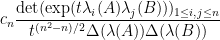
Let 


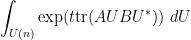
where 


when the eigenvalues of 


and 

There are at least two standard ways to prove this formula in the literature. One way is by applying the Duistermaat-Heckman theorem to the pushforward of Liouville measure on the coadjoint orbit 

The Harish-Chandra-Itzykson-Zuber formula can be extended to other compact Lie groups than 
The 2009 Abel prize has been awarded to Mikhail Gromov, for his contributions to numerous areas of geometry, including Riemannian geometry, symplectic geometry, and geometric group theory.
The prize is, of course, richly deserved. I have mentioned some of Gromov’s work here on this blog, including the Bishop-Gromov inequality in Riemannian geometry (which (together with its parabolic counterpart, the monotonicity of Perelman reduced volume) plays an important role in Perelman’s proof of the Poincaré conjecture), the concept of Gromov-Hausdorff convergence (a version of which is also key in the proof of the Poincaré conjecture), and Gromov’s celebrated theorem on groups of polynomial growth, which I discussed in this post.
Another well-known result of Gromov that I am quite fond of is his nonsqueezing theorem in symplectic geometry (or Hamiltonian mechanics). In its original form, the theorem states that a ball 


I can sketch Gromov’s original proof of the non-squeezing theorem here. The symplectic space 

Now suppose for contradiction that there is a symplectic embedding 


Just as complex structures can be used to define holomorphic functions, almost complex structures can be used to define pseudo-holomorphic or J-holomorphic curves. These are curves of one complex dimension (i.e. two real dimensions, that is to say a surface) which obey the analogue of the Cauchy-Riemann equations in the almost complex setting (i.e. the tangent space of the curve is preserved by J). The theory of such curves was pioneered by Gromov in the paper where the nonsqueezing theorem was proved. When J is the standard almost complex structure on 
Now, the point 


As is well known, the linear one-dimensional wave equation
where 

for some arbitrary (smooth) functions 
When one moves from linear wave equations to nonlinear wave equations, then in general one does not expect to have a closed-form solution such as (2). So I was pleasantly surprised recently while playing with the nonlinear wave equation
to discover that this equation can also be explicitly solved in closed form. (I hope to explain why I was interested in (3) in the first place in a later post.)
A posteriori, I now know the reason for this explicit solvability; (3) is the limiting case 

which (after applying the simple transformation 
(a close cousin of the more famous sine-Gordon equation 
[The computations do seem to be very classical, though, and thus presumably already in the literature; if anyone knows of a place where the solvability of (3) is discussed, I would be very happy to learn of it.] [Update, Jan 22: Patrick Dorey has pointed out that (3) is, indeed, extremely classical; it is known as Liouville’s equation and was solved by Liouville in J. Math. Pure et Appl. vol 18 (1853), 71-74, with essentially the same solution as presented here.]
My penultimate article for my PCM series is a very short one, on “Hamiltonians“. The PCM has a number of short articles to define terms which occur frequently in the longer articles, but are not substantive enough topics by themselves to warrant a full-length treatment. One of these is the term “Hamiltonian”, which is used in all the standard types of physical mechanics (classical or quantum, microscopic or statistical) to describe the total energy of a system. It is a remarkable feature of the laws of physics that this single object (which is a scalar-valued function in classical physics, and a self-adjoint operator in quantum mechanics) suffices to describe the entire dynamics of a system, although from a mathematical perspective it is not always easy to read off all the analytic aspects of this dynamics just from the form of the Hamiltonian.
In mathematics, Hamiltonians of course arise in the equations of mathematical physics (such as Hamilton’s equations of motion, or Schrödinger’s equations of motion), but also show up in symplectic geometry (as a special case of a moment map) and in microlocal analysis.
For this post, I would also like to highlight an article of my good friend Andrew Granville on one of my own favorite topics, “Analytic number theory“, focusing in particular on the classical problem of understanding the distribution of the primes, via such analytic tools as zeta functions and L-functions, sieve theory, and the circle method.

Recent Comments