
You are currently browsing the monthly archive for December 2022.
This post is an unofficial sequel to one of my first blog posts from 2007, which was entitled “Quantum mechanics and Tomb Raider“.
One of the oldest and most famous allegories is Plato’s allegory of the cave. This allegory centers around a group of people chained to a wall in a cave that cannot see themselves or each other, but only the two-dimensional shadows of themselves cast on the wall in front of them by some light source they cannot directly see. Because of this, they identify reality with this two-dimensional representation, and have significant conceptual difficulties in trying to view themselves (or the world as a whole) as three-dimensional, until they are freed from the cave and able to venture into the sunlight.
There is a similar conceptual difficulty when trying to understand Einstein’s theory of special relativity (and more so for general relativity, but let us focus on special relativity for now). We are very much accustomed to thinking of reality as a three-dimensional space endowed with a Euclidean geometry that we traverse through in time, but in order to have the clearest view of the universe of special relativity it is better to think of reality instead as a four-dimensional spacetime that is endowed instead with a Minkowski geometry, which mathematically is similar to a (four-dimensional) Euclidean space but with a crucial change of sign in the underlying metric. Indeed, whereas the distance 


 of that space, and the distance in a four-dimensional Euclidean space
  would be similarly given by
 , the spacetime interval in Minkowski space is given by
 is preferred) in spacetime coordinates
  , where
  is the speed of light. The geometry of Minkowski space is then quite similar algebraically to the geometry of Euclidean space (with the sign change replacing the traditional trigonometric functions
  , etc. by their hyperbolic counterparts
  , and with various factors involving “” inserted in the formulae), but also has some qualitative differences to Euclidean space, most notably a causality structure connected to light cones that has no obvious counterpart in Euclidean space.
That said, the analogy between Minkowski space and four-dimensional Euclidean space is strong enough that it serves as a useful conceptual aid when first learning special relativity; for instance the excellent introductory text “Spacetime physics” by Taylor and Wheeler very much adopts this view. On the other hand, this analogy doesn’t directly address the conceptual problem mentioned earlier of viewing reality as a four-dimensional spacetime in the first place, rather than as a three-dimensional space that objects move around in as time progresses. Of course, part of the issue is that we aren’t good at directly visualizing four dimensions in the first place. This latter problem can at least be easily addressed by removing one or two spatial dimensions from this framework – and indeed many relativity texts start with the simplified setting of only having one spatial dimension, so that spacetime becomes two-dimensional and can be depicted with relative ease by spacetime diagrams – but still there is conceptual resistance to the idea of treating time as another spatial dimension, since we clearly cannot “move around” in time as freely as we can in space, nor do we seem able to easily “rotate” between the spatial and temporal axes, the way that we can between the three coordinate axes of Euclidean space.
With this in mind, I thought it might be worth attempting a Plato-type allegory to reconcile the spatial and spacetime views of reality, in a way that can be used to describe (analogues of) some of the less intuitive features of relativity, such as time dilation, length contraction, and the relativity of simultaneity. I have (somewhat whimsically) decided to place this allegory in a Tolkienesque fantasy world (similarly to how my previous allegory to describe quantum mechanics was phrased in a world based on the computer game “Tomb Raider”). This is something of an experiment, and (like any other analogy) the allegory will not be able to perfectly capture every aspect of the phenomenon it is trying to represent, so any feedback to improve the allegory would be appreciated.
If 


 , or lower tail probabilities
 . A standard tool for this is Bennett’s inequality:
Proposition 1 (Bennett’s inequality) One hasfor
for


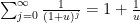
From the Taylor expansion 


Proof: We use the exponential moment method. For any 


 , it turns out that the right-hand side is optimized by setting
  , in which case the right-hand side simplifies to
  . This proves the first inequality; the second inequality is proven similarly (but now and
  are non-positive rather than non-negative).
Remark 2 Bennett’s inequality also applies for (suitably normalized) sums of bounded independent random variables. In some cases there are direct comparison inequalities available to relate those variables to the Poisson case. For instance, supposeis the sum of independent Boolean variables
of total mean
and with
for some
. Then for any natural number
, we have
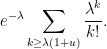
As such, for
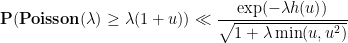
small, one can efficiently control the tail probabilities of
in terms of the tail probability of a Poisson random variable of mean close to


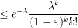

In this note I wanted to record the observation that one can improve the Bennett bound by a small polynomial factor once one leaves the Gaussian regime 

Proposition 3 (Improved Bennett’s inequality) One hasfor
for

Proof: We begin with the first inequality. We may assume that 
 that
that 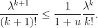
 . We can thus bound the left-hand side by
 for
for  , thus we can bound it by
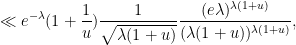
Now we turn to the second inequality. As before we may assume that 


 is negative and
 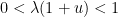 , we see that the right-hand side is
  , and the estimate holds in this case.
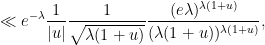
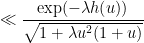
It remains to consider the regime where 

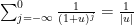 . The maximal is comparable to
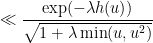
  , so we can bound the left-hand side by
The same analysis can be reversed to show that the bounds given above are basically sharp up to constants, at least when
[The following information was provided to me by Geordie Williamson, who is Director of the Sydney Mathematics Research Institute – T.]
We are currently advertising two positions in math and AI:
- A Level A position (for first time postdocs, upcoming PhDs); and
- a Level B position (for candidates with a postdoc / some research experience):
Both positions are for three years and are based at the Sydney Mathematical Research Institute. The positions are research only, but teaching at the University of Sydney is possible if desired. The successful candidate will have considerable time and flexibility to pursue their own research program.
We are after either:
- excellent mathematicians with some interest in programming and modern AI;
- excellent computer scientists with some interest and background in mathematics, as well as an interest in using AI to attack tough problems in mathematics.

Recent Comments