
You are currently browsing the tag archive for the ‘nonstandard analysis’ tag.
Note: this post is not required reading for this course, or for the sequel course in the winter quarter.
In a Notes 2, we reviewed the classical construction of Leray of global weak solutions to the Navier-Stokes equations. We did not quite follow Leray’s original proof, in that the notes relied more heavily on the machinery of Littlewood-Paley projections, which have become increasingly common tools in modern PDE. On the other hand, we did use the same “exploiting compactness to pass to weakly convergent subsequence” strategy that is the standard one in the PDE literature used to construct weak solutions.
As I discussed in a previous post, the manipulation of sequences and their limits is analogous to a “cheap” version of nonstandard analysis in which one uses the Fréchet filter rather than an ultrafilter to construct the nonstandard universe. (The manipulation of generalised functions of Columbeau-type can also be comfortably interpreted within this sort of cheap nonstandard analysis.) Augmenting the manipulation of sequences with the right to pass to subsequences whenever convenient is then analogous to a sort of “lazy” nonstandard analysis, in which the implied ultrafilter is never actually constructed as a “completed object“, but is instead lazily evaluated, in the sense that whenever membership of a given subsequence of the natural numbers in the ultrafilter needs to be determined, one either passes to that subsequence (thus placing it in the ultrafilter) or the complement of the sequence (placing it out of the ultrafilter). This process can be viewed as the initial portion of the transfinite induction that one usually uses to construct ultrafilters (as discussed using a voting metaphor in this post), except that there is generally no need in any given application to perform the induction for any uncountable ordinal (or indeed for most of the countable ordinals also).
On the other hand, it is also possible to work directly in the orthodox framework of nonstandard analysis when constructing weak solutions. This leads to an approach to the subject which is largely equivalent to the usual subsequence-based approach, though there are some minor technical differences (for instance, the subsequence approach occasionally requires one to work with separable function spaces, whereas in the ultrafilter approach the reliance on separability is largely eliminated, particularly if one imposes a strong notion of saturation on the nonstandard universe). The subject acquires a more “algebraic” flavour, as the quintessential analysis operation of taking a limit is replaced with the “standard part” operation, which is an algebra homomorphism. The notion of a sequence is replaced by the distinction between standard and nonstandard objects, and the need to pass to subsequences disappears entirely. Also, the distinction between “bounded sequences” and “convergent sequences” is largely eradicated, particularly when the space that the sequences ranged in enjoys some compactness properties on bounded sets. Also, in this framework, the notorious non-uniqueness features of weak solutions can be “blamed” on the non-uniqueness of the nonstandard extension of the standard universe (as well as on the multiple possible ways to construct nonstandard mollifications of the original standard PDE). However, many of these changes are largely cosmetic; switching from a subsequence-based theory to a nonstandard analysis-based theory does not seem to bring one significantly closer for instance to the global regularity problem for Navier-Stokes, but it could have been an alternate path for the historical development and presentation of the subject.
In any case, I would like to present below the fold this nonstandard analysis perspective, quickly translating the relevant components of real analysis, functional analysis, and distributional theory that we need to this perspective, and then use it to re-prove Leray’s theorem on existence of global weak solutions to Navier-Stokes.
Read the rest of this entry »
Szemerédi’s theorem asserts that any subset of the integers of positive upper density contains arbitrarily large arithmetic progressions. Here is an equivalent quantitative form of this theorem:
Theorem 1 (Szemerédi’s theorem) Let
be a positive integer, and let
be a function with
for some
, where we use the averaging notation
,
, etc.. Then for
we have
for some
depending only on
.

The equivalence is basically thanks to an averaging argument of Varnavides; see for instance Chapter 11 of my book with Van Vu or this previous blog post for a discussion. We have removed the cases 
There are now many proofs of this theorem. Some time ago, I took an ergodic-theoretic proof of Furstenberg and converted it to a purely finitary proof of the theorem. The argument used some simplifying innovations that had been developed since the original work of Furstenberg (in particular, deployment of the Gowers uniformity norms, as well as a “dual” norm that I called the uniformly almost periodic norm, and an emphasis on van der Waerden’s theorem for handling the “compact extension” component of the argument). But the proof was still quite messy. However, as discussed in this previous blog post, messy finitary proofs can often be cleaned up using nonstandard analysis. Thus, there should be a nonstandard version of the Furstenberg ergodic theory argument that is relatively clean. I decided (after some encouragement from Ben Green and Isaac Goldbring) to write down most of the details of this argument in this blog post, though for sake of brevity I will skim rather quickly over arguments that were already discussed at length in other blog posts. In particular, I will presume familiarity with nonstandard analysis (in particular, the notion of a standard part of a bounded real number, and the Loeb measure construction), see for instance this previous blog post for a discussion.
In graph theory, the recently developed theory of graph limits has proven to be a useful tool for analysing large dense graphs, being a convenient reformulation of the Szemerédi regularity lemma. Roughly speaking, the theory asserts that given any sequence 

![{p\colon [0,1] \times [0,1] \rightarrow [0,1]}](https://s0.wp.com/latex.php?latex=%7Bp%5Ccolon+%5B0%2C1%5D+%5Ctimes+%5B0%2C1%5D+%5Crightarrow+%5B0%2C1%5D%7D&bg=ffffff&fg=000000&s=0&c=20201002)


converge to the integral
the triangle density

converges to the integral

the four-cycle density

converges to the integral

and so forth. One can use graph limits to prove many results in graph theory that were traditionally proven using the regularity lemma, such as the triangle removal lemma, and can also reduce many asymptotic graph theory problems to continuous problems involving multilinear integrals (although the latter problems are not necessarily easy to solve!). See this text of Lovasz for a detailed study of graph limits and their applications.
One can also express graph limits (and more generally hypergraph limits) in the language of nonstandard analysis (or of ultraproducts); see for instance this paper of Elek and Szegedy, Section 6 of this previous blog post, or this paper of Towsner. (In this post we assume some familiarity with nonstandard analysis, as reviewed for instance in the previous blog post.) Here, one starts as before with a sequence 


where the “graphon” 


![{p\colon V_\alpha \times V_\alpha \rightarrow [0,1]}](https://s0.wp.com/latex.php?latex=%7Bp%5Ccolon+V_%5Calpha+%5Ctimes+V_%5Calpha+%5Crightarrow+%5B0%2C1%5D%7D&bg=ffffff&fg=000000&s=0&c=20201002)


(or equivalently, the limit of the 

where 


(or equivalently, the limit along 

and so forth. Note that with this construction, the graphon ![{[0,1]}](https://s0.wp.com/latex.php?latex=%7B%5B0%2C1%5D%7D&bg=ffffff&fg=000000&s=0&c=20201002)
Additive combinatorics, which studies things like the additive structure of finite subsets 

It seems that to allow for the most flexible and powerful manifestation of this theory, it is convenient to use the nonstandard formulation (among other things, it allows for full use of the transfer principle, whereas a more traditional limit formulation would only allow for a transfer of those quantities continuous with respect to the notion of convergence). Here, the analogue of a nonstandard graph is an ultra approximate group 


whenever
The Loeb measure 
- There is not an obvious topology on
- The addition operation
is not measurable from the product Loeb algebra
to
. Instead, it is measurable from the coarser Loeb algebra
to
Nevertheless, the analogy is a useful guide for the arguments that follow.
Let 


whenever 


The basic structural theorem is then as follows.
Theorem 1 (Kronecker factor) Let
of the form
for some standard
and some compact abelian group
, equipped with a Haar measure
and a measurable homomorphism
(using the Loeb
- (i)
has dense image, and
- (ii) There exists sets
with
open and
compact, such that
- (iii) Whenever
with
open, there exists a nonstandard finite set
such that
- (iv) If
, then we have the convolution formula
where
are the pushforwards of
to
, the convolution
on the right-hand side is convolution using
is the pullback map from
to
. In particular, if
, then
for all
.


One can view the locally compact abelian group 

Given any sequence of uniformly bounded functions 


as an “additive limit” of the 


converge (along the ultrafilter

and for three sequences 

converges along
the normalised 

converges along

and so forth. We caution however that some correlations that involve evaluating more than one function at the same point will not necessarily be preserved in the additive limit; for instance the normalised 

does not necessarily converge to the 

but can converge instead to a larger quantity, due to the presence of the orthogonal projection 
An important special case of an additive limit occurs when the functions 


![{f \star f\colon G \rightarrow [0,1]}](https://s0.wp.com/latex.php?latex=%7Bf+%5Cstar+f%5Ccolon+G+%5Crightarrow+%5B0%2C1%5D%7D&bg=ffffff&fg=000000&s=0&c=20201002)


Theorem 1 can be proven by Fourier-analytic means (combined with Freiman’s theorem from additive combinatorics), and we will do so below the fold. For now, we give some illustrative examples of additive limits.
Example 2 (Bohr sets) We take
, where
is a sequence going to infinity; these are
-approximate groups for all
be an irrational real number, let
be an interval in
, and for each natural number
be the Bohr set
In this case, the (reduced) Kronecker factor
with the usual Lebesgue measure
and
end up being
and
, where
and
Geometrically, one should think of
, and then one sees that
to be quadratic in
becomes comparable to
, at which point the growth transitions to linear growth, in the regime where
If
were rational instead of irrational, then one would need to replace
here.

![\displaystyle A := \{ (x,t) \in {\bf R} \times {\bf R}/{\bf Z}: x \in [-1,1]\}](https://s0.wp.com/latex.php?latex=%5Cdisplaystyle++A+%3A%3D+%5C%7B+%28x%2Ct%29+%5Cin+%7B%5Cbf+R%7D+%5Ctimes+%7B%5Cbf+R%7D%2F%7B%5Cbf+Z%7D%3A+x+%5Cin+%5B-1%2C1%5D%5C%7D&bg=ffffff&fg=000000&s=0&c=20201002)
![\displaystyle B := \{ (x,t) \in {\bf R} \times {\bf R}/{\bf Z}: x \in [-1,1]; t \in I \}.](https://s0.wp.com/latex.php?latex=%5Cdisplaystyle++B+%3A%3D+%5C%7B+%28x%2Ct%29+%5Cin+%7B%5Cbf+R%7D+%5Ctimes+%7B%5Cbf+R%7D%2F%7B%5Cbf+Z%7D%3A+x+%5Cin+%5B-1%2C1%5D%3B+t+%5Cin+I+%5C%7D.&bg=ffffff&fg=000000&s=0&c=20201002)
Example 3 (Structured subsets of progressions) We take
where
-approximate groups for all
Then the (reduced) Kronecker factor can be taken to be
with Lebesgue measure
and
Geometrically, the picture is similar to the Bohr set one, except now one uses a Freiman homomorphism
for
to embed the original sets
into the plane
. In particular, one now expects the growth rate of the iterated sumsets
and
to be quadratic in


Example 4 (Dissociated sets) Let
be a fixed natural number, and take
where
are randomly chosen elements of a large cyclic group
, where
is a sequence of primes going to infinity. These are
-approximate groups. The (reduced) Kronecker factor
with counting measure, and the additive limit of
and
is the standard basis of
for

Example 5 (Random subsets of groups) Let
be a sequence of finite additive groups whose order is going to infinity. Let
of some fixed density
. Then (almost surely) the Kronecker factor here can be reduced all the way to the trivial group
, and the additive limit of the
. The convolutions
then converge in the ultralimit (modulo almost everywhere equivalence) to the pullback of
; this reflects the fact that
of the elements of
ways. In particular,
occupies a proportion
of
Example 6 (Trigonometric series) Take
for a sequence
be an infinite sequence of frequencies chosen uniformly and independently from
denote the random trigonometric series
Then (almost surely) we can take the reduced Kronecker factor
(with the Haar probability measure
defined by the formula
In fact, the pullback
is the ultralimit of the
, the normalised
norm
can be seen to converge to the limit


The reader is invited to consider combinations of the above examples, e.g. random subsets of Bohr sets, to get a sense of the general case of Theorem 1.
It is likely that this theorem can be extended to the noncommutative setting, using the noncommutative Freiman theorem of Emmanuel Breuillard, Ben Green, and myself, but I have not attempted to do so here (see though this recent preprint of Anush Tserunyan for some related explorations); in a separate direction, there should be extensions that can control higher Gowers norms, in the spirit of the work of Szegedy.
Note: the arguments below will presume some familiarity with additive combinatorics and with nonstandard analysis, and will be a little sketchy in places.
Let 


Let 


for the irrationality of 


from which the bound (1) easily follows. A well known corollary of the bound (1) is that Liouville numbers are automatically transcendental.
The famous theorem of Thue, Siegel and Roth improves the bound (1) to

for any 


A powerful strengthening of the Thue-Siegel-Roth theorem is given by the subspace theorem, first proven by Schmidt and then generalised further by several authors. To motivate the theorem, first observe that the Thue-Siegel-Roth theorem may be rephrased as a bound of the form

for any algebraic numbers 


Theorem 1 (Schmidt subspace theorem) Let
be linearly independent linear forms. Then for any
for all
, outside of a finite number of proper subspaces of
, where
and
and the
, but is independent of
.

Being a generalisation of the Thue-Siegel-Roth theorem, it is unsurprising that the known proofs of the subspace theorem are also ineffective with regards to the constant 


![{x_1,\dots,x_d \in [-N,N]}](https://s0.wp.com/latex.php?latex=%7Bx_1%2C%5Cdots%2Cx_d+%5Cin+%5B-N%2CN%5D%7D&bg=ffffff&fg=000000&s=0&c=20201002)

for all 

There are important generalisations of the subspace theorem to other number fields than the rationals (and to other valuations than the Archimedean valuation
The subspace theorem is one of many finiteness theorems in Diophantine geometry; in this case, it is the number of exceptional subspaces which is finite. It turns out that finiteness theorems are very compatible with the language of nonstandard analysis. (See this previous blog post for a review of the basics of nonstandard analysis, and in particular for the nonstandard interpretation of asymptotic notation such as 


Theorem 2 (Bezout’s theorem, nonstandard form) Let
.
Now we reformulate Theorem 1 in nonstandard language. We need a definition:
Definition 3 (General position) Let
be nested fields. A point
in
is said to be in
for any
.

Theorem 4 (Schmidt subspace theorem, nonstandard version) Let
be a tuple of nonstandard integers which is in
where we extend
from
(and also similarly extend
from
) in the usual fashion.

Observe that (as is usual when translating to nonstandard analysis) some of the epsilons and quantifiers that are present in the standard version become hidden in the nonstandard framework, being moved inside concepts such as “strictly nonstandard” or “general position”. We remark that as 

Exercise 1 Verify that Theorem 1 and Theorem 4 are equivalent. (Hint: there are only countably many proper subspaces of
We will not prove the subspace theorem here, but instead focus on a particular application of the subspace theorem, namely to counting integer points on curves. In this paper of Corvaja and Zannier, the subspace theorem was used to give a new proof of the following basic result of Siegel:
Theorem 5 (Siegel’s theorem on integer points) Let
be an irreducible polynomial of two variables, such that the affine plane curve
either has genus at least one, or has at least three points on the line at infinity, or both. Then
has only finitely many integer points
.
This is a finiteness theorem, and as such may be easily converted to a nonstandard form:
Theorem 6 (Siegel’s theorem, nonstandard form) Let
.
Note that Siegel’s theorem can fail for genus zero curves that only meet the line at infinity at just one or two points; the key examples here are the graphs 
![{f \in {\bf Z}[x]}](https://s0.wp.com/latex.php?latex=%7Bf+%5Cin+%7B%5Cbf+Z%7D%5Bx%5D%7D&bg=ffffff&fg=000000&s=0&c=20201002)

The standard proofs of Siegel’s theorem rely on a combination of the Thue-Siegel-Roth theorem and a number of results on abelian varieties (notably the Mordell-Weil theorem). The Corvaja-Zannier argument rebalances the difficulty of the argument by replacing the Thue-Siegel-Roth theorem by the more powerful subspace theorem (in fact, they need one of the stronger versions of this theorem alluded to earlier), while greatly reducing the reliance on results on abelian varieties. Indeed, for curves with three or more points at infinity, no theory from abelian varieties is needed at all, while for the remaining cases, one mainly needs the existence of the Abel-Jacobi embedding, together with a relatively elementary theorem of Chevalley-Weil which is used in the proof of the Mordell-Weil theorem, but is significantly easier to prove.
The Corvaja-Zannier argument (together with several further applications of the subspace theorem) is presented nicely in this Bourbaki expose of Bilu. To establish the theorem in full generality requires a certain amount of algebraic number theory machinery, such as the theory of valuations on number fields, or of relative discriminants between such number fields. However, the basic ideas can be presented without much of this machinery by focusing on simple special cases of Siegel’s theorem. For instance, we can handle irreducible cubics that meet the line at infinity at exactly three points ![{[1,\alpha_1,0], [1,\alpha_2,0], [1,\alpha_3,0]}](https://s0.wp.com/latex.php?latex=%7B%5B1%2C%5Calpha_1%2C0%5D%2C+%5B1%2C%5Calpha_2%2C0%5D%2C+%5B1%2C%5Calpha_3%2C0%5D%7D&bg=ffffff&fg=000000&s=0&c=20201002)
Theorem 7 (Siegel’s theorem with three points at infinity) Siegel’s theorem holds when the irreducible polynomial
takes the form
for some quadratic polynomial
and some distinct algebraic numbers
.

Proof: We use the nonstandard formalism. Suppose for sake of contradiction that we can find a strictly nonstandard integer point 

We now use a version of the polynomial method, to find some polynomials of controlled degree that vanish to high order on the “arm” of the cubic curve ![{[1,\alpha_1,0]}](https://s0.wp.com/latex.php?latex=%7B%5B1%2C%5Calpha_1%2C0%5D%7D&bg=ffffff&fg=000000&s=0&c=20201002)


![{R(x,y) \in \bar{{\bf Q}}[x,y]}](https://s0.wp.com/latex.php?latex=%7BR%28x%2Cy%29+%5Cin+%5Cbar%7B%7B%5Cbf+Q%7D%7D%5Bx%2Cy%5D%7D&bg=ffffff&fg=000000&s=0&c=20201002)


From the control of the pole at

for all 

This exponent is negative for
for some algebraic numbers 

for some standard 


for some standard rational coefficients 


Exercise 2 Rewrite the above argument so that it makes no reference to nonstandard analysis. (In this case, the rewriting is quite straightforward; however, there will be a subsequent argument in which the standard version is significantly messier than the nonstandard counterpart, which is the reason why I am working with the nonstandard formalism in this blog post.)
A similar argument works for higher degree curves that meet the line at infinity in three or more points, though if the curve has singularities at infinity then it becomes convenient to rely on the Riemann-Roch theorem to control the dimension of the analogue of the space 

Theorem 8 (Siegel’s theorem for Mordell curves) Let
. More generally, for any number field
, there are only finitely many algebraic integer solutions
to
, where
is the ring of algebraic integers in
Again, we will establish the nonstandard version. We need some additional notation:
Definition 9
We define an almost rational integer to be a nonstandard such that
for some standard positive integer
, and write
for the
If such that
for some standard positive integer
for the
We define an almost algebraic integer to be a nonstandard such that
is a nonstandard algebraic integer for some standard positive integer
for the
Theorem 10 (Siegel for Mordell, nonstandard version) Let
does not contain any strictly nonstandard almost algebraic integer point.
Another way of phrasing this theorem is that if 

Exercise 3 Verify that Theorem 8 and Theorem 10 are equivalent.
Due to all the ineffectivity, our proof does not supply any bound on the solutions 

A direct repetition of the arguments used to prove Theorem 7 will not work here, because the Mordell curve ![{[0,1,0]}](https://s0.wp.com/latex.php?latex=%7B%5B0%2C1%2C0%5D%7D&bg=ffffff&fg=000000&s=0&c=20201002)
There are a number of ways to construct the real numbers 
- as the metric completion of
- as the space of Dedekind cuts on the rationals
- as the space of quasimorphisms
on the integers, quotiented by bounded functions. (I believe this construction first appears in this paper of Street, who credits the idea to Schanuel, though the germ of this construction arguably goes all the way back to Eudoxus.)
There is also a fourth family of constructions that proceeds via nonstandard analysis, as a special case of what is known as the nonstandard hull construction. (Here I will assume some basic familiarity with nonstandard analysis and ultraproducts, as covered for instance in this previous blog post.) Given an unbounded nonstandard natural number 

- The group
of all nonstandard integers of magnitude less than or comparable to
- The group
of nonstandard integers of magnitude infinitesimally smaller than
The group 


Proposition 1 For any coset
of
with the property that
. The map
is then an isomorphism between the additive groups
Proof: Uniqueness is clear. For existence, observe that the set 
In a similar vein, we can view the unit interval
![\displaystyle [0,1] \equiv [N] / o(N) \ \ \ \ \ (1)](https://s0.wp.com/latex.php?latex=%5Cdisplaystyle++%5B0%2C1%5D+%5Cequiv+%5BN%5D+%2F+o%28N%29+%5C+%5C+%5C+%5C+%5C+%281%29&bg=ffffff&fg=000000&s=0&c=20201002)
where ![{[N]}](https://s0.wp.com/latex.php?latex=%7B%5BN%5D%7D&bg=ffffff&fg=000000&s=0&c=20201002)
![{[N]/o(N)}](https://s0.wp.com/latex.php?latex=%7B%5BN%5D%2Fo%28N%29%7D&bg=ffffff&fg=000000&s=0&c=20201002)


In this post I would like to record a nice measure-theoretic version of the equivalence (1), which essentially appears already in standard texts on Loeb measure (see e.g. this text of Cutland). To describe the results, we must first quickly recall the construction of Loeb measure on 

This is a finitely additive probability measure on the Boolean algebra of internal subsets of 
![{A \subset [N]}](https://s0.wp.com/latex.php?latex=%7BA+%5Csubset+%5BN%5D%7D&bg=ffffff&fg=000000&s=0&c=20201002)
where 


![{([N], {\mathcal L}, \mu)}](https://s0.wp.com/latex.php?latex=%7B%28%5BN%5D%2C+%7B%5Cmathcal+L%7D%2C+%5Cmu%29%7D&bg=ffffff&fg=000000&s=0&c=20201002)
Now, the group 
![{n \in [N]}](https://s0.wp.com/latex.php?latex=%7Bn+%5Cin+%5BN%5D%7D&bg=ffffff&fg=000000&s=0&c=20201002)


![{Z^0_{o(N)}([N]) = ([N], {\mathcal L}^{o(N)}, \mu\downharpoonright_{{\mathcal L}^{o(N)}})}](https://s0.wp.com/latex.php?latex=%7BZ%5E0_%7Bo%28N%29%7D%28%5BN%5D%29+%3D+%28%5BN%5D%2C+%7B%5Cmathcal+L%7D%5E%7Bo%28N%29%7D%2C+%5Cmu%5Cdownharpoonright_%7B%7B%5Cmathcal+L%7D%5E%7Bo%28N%29%7D%7D%29%7D&bg=ffffff&fg=000000&s=0&c=20201002)

The claim is then that this invariant factor is equivalent (up to almost everywhere equivalence) to the unit interval
Theorem 2 Given a set
, there exists a Lebesgue measurable set
, unique up to
. Conversely, if
is Lebesgue measurable, then
is in
, and
.
More informally, we have the measure-theoretic version
![\displaystyle [0,1] \equiv Z^0_{o(N)}( [N] )](https://s0.wp.com/latex.php?latex=%5Cdisplaystyle++%5B0%2C1%5D+%5Cequiv+Z%5E0_%7Bo%28N%29%7D%28+%5BN%5D+%29&bg=ffffff&fg=000000&s=0&c=20201002)
of (1).
Proof: We first prove the converse. It is clear that 


![{E \subset [0,1]}](https://s0.wp.com/latex.php?latex=%7BE+%5Csubset+%5B0%2C1%5D%7D&bg=ffffff&fg=000000&s=0&c=20201002)
Now we establish the forward claim. Uniqueness is clear from the converse claim, so it suffices to show existence. Let ![{A_\epsilon \subset [N]}](https://s0.wp.com/latex.php?latex=%7BA_%5Cepsilon+%5Csubset+%5BN%5D%7D&bg=ffffff&fg=000000&s=0&c=20201002)


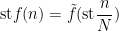
![{f_\epsilon: [N] \rightarrow {}^* {\bf R}}](https://s0.wp.com/latex.php?latex=%7Bf_%5Cepsilon%3A+%5BN%5D+%5Crightarrow+%7B%7D%5E%2A+%7B%5Cbf+R%7D%7D&bg=ffffff&fg=000000&s=0&c=20201002)
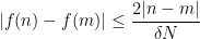
![\displaystyle f(n) := \hbox{st} \frac{1}{\delta N} \sum_{m \in [N]: m \leq n \leq m+\delta N} 1_{A_\epsilon}(m),](https://s0.wp.com/latex.php?latex=%5Cdisplaystyle++f%28n%29+%3A%3D+%5Chbox%7Bst%7D+%5Cfrac%7B1%7D%7B%5Cdelta+N%7D+%5Csum_%7Bm+%5Cin+%5BN%5D%3A+m+%5Cleq+n+%5Cleq+m%2B%5Cdelta+N%7D+1_%7BA_%5Cepsilon%7D%28m%29%2C&bg=ffffff&fg=000000&s=0&c=20201002)
then from the (nonstandard) triangle inequality we have
![\displaystyle \frac{1}{N} \sum_{n \in [N]} |f(n) - 1_{A_\epsilon}(n)| \leq 3\epsilon](https://s0.wp.com/latex.php?latex=%5Cdisplaystyle++%5Cfrac%7B1%7D%7BN%7D+%5Csum_%7Bn+%5Cin+%5BN%5D%7D+%7Cf%28n%29+-+1_%7BA_%5Cepsilon%7D%28n%29%7C+%5Cleq+3%5Cepsilon&bg=ffffff&fg=000000&s=0&c=20201002)
(say). On the other hand,
and so in particular we see that
for some Lipschitz continuous function ![{\tilde f: [0,1] \rightarrow [0,1]}](https://s0.wp.com/latex.php?latex=%7B%5Ctilde+f%3A+%5B0%2C1%5D+%5Crightarrow+%5B0%2C1%5D%7D&bg=ffffff&fg=000000&s=0&c=20201002)


Thanks to the Lebesgue differentiation theorem, the conditional expectation ![{{\bf E}( f | Z^0_{o(N)}([N]))}](https://s0.wp.com/latex.php?latex=%7B%7B%5Cbf+E%7D%28+f+%7C+Z%5E0_%7Bo%28N%29%7D%28%5BN%5D%29%29%7D&bg=ffffff&fg=000000&s=0&c=20201002)
![{f: [N] \rightarrow {\bf R}}](https://s0.wp.com/latex.php?latex=%7Bf%3A+%5BN%5D+%5Crightarrow+%7B%5Cbf+R%7D%7D&bg=ffffff&fg=000000&s=0&c=20201002)
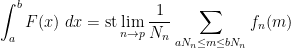
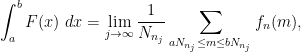
![\displaystyle {\bf E}( f | Z^0_{o(N)}([N]))(x) := \lim_{\epsilon \rightarrow 0} \frac{1}{2\epsilon} \int_{[x-\epsilon N,x+\epsilon N]} f\ d\mu.](https://s0.wp.com/latex.php?latex=%5Cdisplaystyle++%7B%5Cbf+E%7D%28+f+%7C+Z%5E0_%7Bo%28N%29%7D%28%5BN%5D%29%29%28x%29+%3A%3D+%5Clim_%7B%5Cepsilon+%5Crightarrow+0%7D+%5Cfrac%7B1%7D%7B2%5Cepsilon%7D+%5Cint_%7B%5Bx-%5Cepsilon+N%2Cx%2B%5Cepsilon+N%5D%7D+f%5C+d%5Cmu.&bg=ffffff&fg=000000&s=0&c=20201002)
By the abstract ergodic theorem from the previous post, one can also view this conditional expectation as the element in the closed convex hull of the shifts 


If ![{f: [N] \rightarrow [-1,1]}](https://s0.wp.com/latex.php?latex=%7Bf%3A+%5BN%5D+%5Crightarrow+%5B-1%2C1%5D%7D&bg=ffffff&fg=000000&s=0&c=20201002)
![{f_n: [N_n] \rightarrow [-1,1]}](https://s0.wp.com/latex.php?latex=%7Bf_n%3A+%5BN_n%5D+%5Crightarrow+%5B-1%2C1%5D%7D&bg=ffffff&fg=000000&s=0&c=20201002)
![{F := {\bf E}( f | Z^0_{o(N)}([N]))}](https://s0.wp.com/latex.php?latex=%7BF+%3A%3D+%7B%5Cbf+E%7D%28+f+%7C+Z%5E0_%7Bo%28N%29%7D%28%5BN%5D%29%29%7D&bg=ffffff&fg=000000&s=0&c=20201002)
![{F: [0,1] \rightarrow [-1,1]}](https://s0.wp.com/latex.php?latex=%7BF%3A+%5B0%2C1%5D+%5Crightarrow+%5B-1%2C1%5D%7D&bg=ffffff&fg=000000&s=0&c=20201002)
for all 

thus 
![{[N_n]}](https://s0.wp.com/latex.php?latex=%7B%5BN_n%5D%7D&bg=ffffff&fg=000000&s=0&c=20201002)

I’m continuing to look into understanding the ergodic theory of
(This is an extended blog post version of my talk “Ultraproducts as a Bridge Between Discrete and Continuous Analysis” that I gave at the Simons institute for the theory of computing at the workshop “Neo-Classical methods in discrete analysis“. Some of the material here is drawn from previous blog posts, notably “Ultraproducts as a bridge between hard analysis and soft analysis” and “Ultralimit analysis and quantitative algebraic geometry“‘. The text here has substantially more details than the talk; one may wish to skip all of the proofs given here to obtain a closer approximation to the original talk.)
Discrete analysis, of course, is primarily interested in the study of discrete (or “finitary”) mathematical objects: integers, rational numbers (which can be viewed as ratios of integers), finite sets, finite graphs, finite or discrete metric spaces, and so forth. However, many powerful tools in mathematics (e.g. ergodic theory, measure theory, topological group theory, algebraic geometry, spectral theory, etc.) work best when applied to continuous (or “infinitary”) mathematical objects: real or complex numbers, manifolds, algebraic varieties, continuous topological or metric spaces, etc. In order to apply results and ideas from continuous mathematics to discrete settings, there are basically two approaches. One is to directly discretise the arguments used in continuous mathematics, which often requires one to keep careful track of all the bounds on various quantities of interest, particularly with regard to various error terms arising from discretisation which would otherwise have been negligible in the continuous setting. The other is to construct continuous objects as limits of sequences of discrete objects of interest, so that results from continuous mathematics may be applied (often as a “black box”) to the continuous limit, which then can be used to deduce consequences for the original discrete objects which are quantitative (though often ineffectively so). The latter approach is the focus of this current talk.
The following table gives some examples of a discrete theory and its continuous counterpart, together with a limiting procedure that might be used to pass from the former to the latter:
| (Discrete) | (Continuous) | (Limit method) |
| Ramsey theory | Topological dynamics | Compactness |
| Density Ramsey theory | Ergodic theory | Furstenberg correspondence principle |
| Graph/hypergraph regularity | Measure theory | Graph limits |
| Polynomial regularity | Linear algebra | Ultralimits |
| Structural decompositions | Hilbert space geometry | Ultralimits |
| Fourier analysis | Spectral theory | Direct and inverse limits |
| Quantitative algebraic geometry | Algebraic geometry | Schemes |
| Discrete metric spaces | Continuous metric spaces | Gromov-Hausdorff limits |
| Approximate group theory | Topological group theory | Model theory |
As the above table illustrates, there are a variety of different ways to form a limiting continuous object. Roughly speaking, one can divide limits into three categories:
- Topological and metric limits. These notions of limits are commonly used by analysts. Here, one starts with a sequence (or perhaps a net) of objects
in a common space
, which remains in the same space, and is “close” to many of the original objects
- Categorical limits. These notions of limits are commonly used by algebraists. Here, one starts with a sequence (or more generally, a diagram) of objects
or the inverse limit
of these objects, which is another object in the same category
- Logical limits. These notions of limits are commonly used by model theorists. Here, one starts with a sequence of objects
or of spaces
, each of which is (a component of) a model for given (first-order) mathematical language (e.g. if one is working in the language of groups,
or a new space
, which is still a model of the same language (e.g. if the spaces
.)
The purpose of this talk is to highlight the third type of limit, and specifically the ultraproduct construction, as being a “universal” limiting procedure that can be used to replace most of the limits previously mentioned. Unlike the topological or metric limits, one does not need the original objects
With so few requirements on the objects
Ultraproducts are not the only logical limit in the model theorist’s toolbox, but they are one of the simplest to set up and use, and already suffice for many of the applications of logical limits outside of model theory. In this post, I will set out the basic theory of these ultraproducts, and illustrate how they can be used to pass between discrete and continuous theories in each of the examples listed in the above table.
Apart from the initial “one-time cost” of setting up the ultraproduct machinery, the main loss one incurs when using ultraproduct methods is that it becomes very difficult to extract explicit quantitative bounds from results that are proven by transferring qualitative continuous results to the discrete setting via ultraproducts. However, in many cases (particularly those involving regularity-type lemmas) the bounds are already of tower-exponential type or worse, and there is arguably not much to be lost by abandoning the explicit quantitative bounds altogether.
The rectification principle in arithmetic combinatorics asserts, roughly speaking, that very small subsets (or, alternatively, small structured subsets) of an additive group or a field of large characteristic can be modeled (for the purposes of arithmetic combinatorics) by subsets of a group or field of zero characteristic, such as the integers 
Proposition 1 (Additive rectification) Let
for some prime
be an integer. Suppose that
. Then there exists a map
into a subset
of the integers which is a Freiman isomorphism of order
in the sense that for any
, one has
if and only if
Furthermore
is a right-inverse of the obvious projection homomorphism from


The original version of the rectification principle allowed the sets involved to be substantially larger in size (cardinality up to a small constant multiple of
The proof of Proposition 1 is quite short (see Theorem 3.1 of Bilu-Lev-Ruzsa); the main idea is to use Minkowski’s theorem to find a non-trivial dilate 
Very recently, Codrut Grosu obtained an arithmetic analogue of the above theorem, in which the rectification map
Theorem 2 (Arithmetic rectification) Let
for some prime
, and let
. Then there exists a map
and any polynomial
of degree at most
if and only if


Note that it is necessary to use an algebraically closed field such as 

Using Theorem 2, one can transfer results in arithmetic combinatorics (e.g. sum-product or Szemerédi-Trotter type theorems) regarding finite subsets of
Grosu’s argument uses some quantitative elimination theory, and in particular a quantitative variant of a lemma of Chang that was discussed previously on this blog. In that previous blog post, it was observed that (an ineffective version of) Chang’s theorem could be obtained using only qualitative algebraic geometry (as opposed to quantitative algebraic geometry tools such as elimination theory results with explicit bounds) by means of nonstandard analysis (or, in what amounts to essentially the same thing in this context, the use of ultraproducts). One can then ask whether one can similarly establish an ineffective version of Grosu’s result by nonstandard means. The purpose of this post is to record that this can indeed be done without much difficulty, though the result obtained, being ineffective, is somewhat weaker than that in Theorem 2. More precisely, we obtain
Theorem 3 (Ineffective arithmetic rectification) Let
. Then if
is a field of characteristic at least
for some
, and
Our arguments will not provide any effective bound on the quantity
Following the principle that ultraproducts can be used as a bridge to connect quantitative and qualitative results (as discussed in these previous blog posts), we will deduce Theorem 3 from the following (well-known) qualitative version:
Proposition 4 (Baby Lefschetz principle) Let
from
of
This principle (first laid out in an appendix of Lefschetz’s book), among other things, often allows one to use the methods of complex analysis (e.g. Riemann surface theory) to study many other fields of characteristic zero. There are many variants and extensions of this principle; see for instance this MathOverflow post for some discussion of these. I used this baby version of the Lefschetz principle recently in a paper on expanding polynomial maps.
Proof: We give two proofs of this fact, one using transcendence bases and the other using Hilbert’s nullstellensatz.
We begin with the former proof. As 


Now we give the latter proof. Let 
if and only if

Let 


is the intersection of countably many algebraic sets and is thus also an algebraic set (by the Hilbert basis theorem or the Noetherian property of algebraic sets). If the desired claim failed, then 


for some 

for some natural numbers 


From Proposition 4 one can now deduce Theorem 3 by a routine ultraproduct argument (the same one used in these previous blog posts). Suppose for contradiction that Theorem 3 fails. Then there exists natural numbers 


Now let 


if and only if

By Los’s theorem, we then conclude that for all
if and only if
But this gives a Freiman field isomorphism of order 
Two weeks ago I was at Oberwolfach, for the Arbeitsgemeinschaft in Ergodic Theory and Combinatorial Number Theory that I was one of the organisers for. At this workshop, I learned the details of a very nice recent convergence result of Miguel Walsh (who, incidentally, is an informal grandstudent of mine, as his advisor, Roman Sasyk, was my informal student), which considerably strengthens and generalises a number of previous convergence results in ergodic theory (including one of my own), with a remarkably simple proof. Walsh’s argument is phrased in a finitary language (somewhat similar, in fact, to the approach used in my paper mentioned previously), and (among other things) relies on the concept of metastability of sequences, a variant of the notion of convergence which is useful in situations in which one does not expect a uniform convergence rate; see this previous blog post for some discussion of metastability. When interpreted in a finitary setting, this concept requires a fair amount of “epsilon management” to manipulate; also, Walsh’s argument uses some other epsilon-intensive finitary arguments, such as a decomposition lemma of Gowers based on the Hahn-Banach theorem. As such, I was tempted to try to rewrite Walsh’s argument in the language of nonstandard analysis to see the extent to which these sorts of issues could be managed. As it turns out, the argument gets cleaned up rather nicely, with the notion of metastability being replaced with the simpler notion of external Cauchy convergence (which we will define below the fold).
Let’s first state Walsh’s theorem. This theorem is a norm convergence theorem in ergodic theory, and can be viewed as a substantial generalisation of one of the most fundamental theorems of this type, namely the mean ergodic theorem:
Theorem 1 (Mean ergodic theorem) Let
be a measure-preserving system (a probability space
with an invertible measure-preserving transformation
, the averages
converge in
norm as
, where
.
In this post, all functions in
Actually, we have a precise description of the limit of these averages, namely the orthogonal projection of
Theorem 2 (von Neumann mean ergodic theorem) Let
be a Hilbert space, and let
be a unitary operator on
, the averages
converge strongly in
Again, see my lecture notes (or just about any text in ergodic theory) for a proof.
Now we turn to Walsh’s theorem.
Theorem 3 (Walsh’s convergence theorem) Let
be polynomial sequences in
takes the form
for some
and polynomials
). Then for any
, the averages
converge in
.
It turns out that this theorem can also be abstracted to some extent, although due to the multiplication in the summand 


Given a commutative probability space, we can form an inner product 

This is a positive semi-definite form, and gives a (possibly degenerate) inner product structure on 


for any
The abstract version of Theorem 3 is then
Theorem 4 (Walsh’s theorem, abstract version) Let
, the averages
It is easy to see that this theorem generalises Theorem 3. Conversely, one can use the commutative Gelfand-Naimark theorem to deduce Theorem 4 from Theorem 3, although we will not need this implication. Note how we are abandoning all attempts to discern what the limit of the sequence actually is, instead contenting ourselves with demonstrating that it is merely a Cauchy sequence. With this phrasing, it is tempting to ask whether there is any analogue of Walsh’s theorem for noncommutative probability spaces, but unfortunately the answer to that question is negative for all but the simplest of averages, as was worked out in this paper of Austin, Eisner, and myself.
Our proof of Theorem 4 will proceed as follows. Firstly, in order to avoid the epsilon management alluded to earlier, we will take an ultraproduct to rephrase the theorem in the language of nonstandard analysis; for reasons that will be clearer later, we will also convert the convergence problem to a problem of obtaining metastability (external Cauchy convergence). Then, we observe that (the nonstandard counterpart of) the expression 


Much as group theory is the study of groups, or graph theory is the study of graphs, model theory is the study of models (also known as structures) of some language
We will observe the common abuse of notation of using the set 


Once one has a structure 


for some formula 


In the theory of the field of reals 


but so is the the complement of the circle,

and the interval ![{[-1,1]}](https://s0.wp.com/latex.php?latex=%7B%5B-1%2C1%5D%7D&bg=ffffff&fg=000000&s=0&c=20201002)
![\displaystyle [-1,1] = \{ x \in {\bf R}: \exists y: x^2+y^2 = 1\}.](https://s0.wp.com/latex.php?latex=%5Cdisplaystyle++%5B-1%2C1%5D+%3D+%5C%7B+x+%5Cin+%7B%5Cbf+R%7D%3A+%5Cexists+y%3A+x%5E2%2By%5E2+%3D+1%5C%7D.&bg=ffffff&fg=000000&s=0&c=20201002)
Due to the unlimited use of constants, any finite subset of a power 
We can isolate some special subclasses of definable sets:
- An atomic definable set is a set of the form (1) in which
is an atomic formula (i.e. it does not contain any logical connectives or quantifiers).
- A quantifier-free definable set is a set of the form (1) in which
Example 1 In the theory of a field such as
.
A quantifier-free definable set in 


Some structures have the property of enjoying quantifier elimination, which means that every definable set is in fact a quantifier-free definable set, or equivalently that the projection of a quantifier-free definable set is again quantifier-free. For instance, an algebraically closed field 

On the other hand, many important structures do not have quantifier elimination; typically, the projection of a quantifier-free definable set is not, in general, quantifier-free definable. This failure of the projection property also shows up in many contexts outside of model theory; for instance, Lebesgue famously made the error of thinking that the projection of a Borel measurable set remained Borel measurable (it is merely an analytic set instead). Turing’s halting theorem can be viewed as an assertion that the projection of a decidable set (also known as a computable or recursive set) is not necessarily decidable (it is merely semi-decidable (or recursively enumerable) instead). The notorious P=NP problem can also be essentially viewed in this spirit; roughly speaking (and glossing over the placement of some quantifiers), it asks whether the projection of a polynomial-time decidable set is again polynomial-time decidable. And so forth. (See this blog post of Dick Lipton for further discussion of the subtleties of projections.)
Now we consider the status of quantifier elimination for the theory of a finite field 


Another way to proceed is to work not with a single finite field 


The ultraproduct
As mentioned before, quantifier elimination trivially holds for finite fields. But for infinite pseudo-finite fields, such as the ultraproduct 


Nevertheless, there is a very nice almost quantifier elimination result for these fields, in characteristic zero at least, which we phrase here as follows:
Theorem 1 (Almost quantifier elimination) Let
be a definable set over
where
is an atomic definable subset of
is a polynomial.

Results of this type were first obtained essentially due to Catarina Kiefe, although the formulation here is closer to that of Chatzidakis-van den Dries-Macintyre.
Informally, this theorem says that while we cannot quite eliminate all quantifiers from a definable set over a nonstandard finite field, we can eliminate all but one existential quantifier. Note that negation has also been eliminated in this theorem; for instance, the definable set 


There is an equivalent formulation of this theorem for standard finite fields, namely that if 

The theorem gives quite a satisfactory description of definable sets in either standard or nonstandard finite fields (at least if one does not care about effective bounds in some of the constants, and if one is willing to exclude the small characteristic case); for instance, in conjunction with the Lang-Weil bound discussed in this recent blog post, it shows that any non-empty definable subset of a nonstandard finite field has a nonstandard cardinality of 

Below the fold I give a proof of Theorem 1, which relies primarily on the Lang-Weil bound mentioned above.
Nonstandard analysis is a mathematical framework in which one extends the standard mathematical universe 

To build a nonstandard universe
On the other hand, nonprincipal ultrafilters do have some unappealing features. The most notable one is that their very existence requires the axiom of choice (or more precisely, a weaker form of this axiom known as the boolean prime ideal theorem). Closely related to this is the fact that one cannot actually write down any explicit example of a nonprincipal ultrafilter, but must instead rely on nonconstructive tools such as Zorn’s lemma, the Hahn-Banach theorem, Tychonoff’s theorem, the Stone-Cech compactification, or the boolean prime ideal theorem to locate one. As such, ultrafilters definitely belong to the “infinitary” side of mathematics, and one may feel that it is inappropriate to use such tools for “finitary” mathematical applications, such as those which arise in hard analysis. From a more practical viewpoint, because of the presence of the infinitary ultrafilter, it can be quite difficult (though usually not impossible, with sufficient patience and effort) to take a finitary result proven via nonstandard analysis and coax an effective quantitative bound from it.
There is however a “cheap” version of nonstandard analysis which is less powerful than the full version, but is not as infinitary in that it is constructive (in the sense of not requiring any sort of choice-type axiom), and which can be translated into standard analysis somewhat more easily than a fully nonstandard argument; indeed, a cheap nonstandard argument can often be presented (by judicious use of asymptotic notation) in a way which is nearly indistinguishable from a standard one. It is obtained by replacing the nonprincipal ultrafilter in fully nonstandard analysis with the more classical Fréchet filter of cofinite subsets of the natural numbers, which is the filter that implicitly underlies the concept of the classical limit 


Below the fold, I would like to describe this cheap version of nonstandard analysis, which I think can serve as a pedagogical stepping stone towards fully nonstandard analysis, as it is formally similar to (though weaker than) fully nonstandard analysis, but on the other hand is closer in practice to standard analysis. As we shall see below, the relation between cheap nonstandard analysis and standard analysis is analogous in many ways to the relation between probabilistic reasoning and deterministic reasoning; it also resembles somewhat the preference in much of modern mathematics for viewing mathematical objects as belonging to families (or to categories) to be manipulated en masse, rather than treating each object individually. (For instance, nonstandard analysis can be used as a partial substitute for scheme theory in order to obtain uniformly quantitative results in algebraic geometry, as discussed for instance in this previous blog post.)

Recent Comments