Erratum for “An inverse theorem for the Gowers U^{s+1}[N]-norm”

The purpose of this post is to report an erratum to the 2012 paper “An inverse theorem for the Gowers -norm” of Ben Green, myself, and Tamar Ziegler (previously discussed in this blog post). The main results of this paper have been superseded with stronger quantitative results, first in work of Manners (using somewhat different methods), and more recently in a remarkable paper of Leng, Sah, and Sawhney which combined the methods of our paper with several new innovations to obtain quite strong bounds (of quasipolynomial type); see also an alternate proof of our main results (again by quite different methods) by Candela and Szegedy. In the course of their work, they discovered some fixable but nontrivial errors in our paper. These (rather technical) issues were already implicitly corrected in this followup work which supersedes our own paper, but for the sake of completeness we are also providing a formal erratum for our original paper, which can be found here. We thank Leng, Sah, and Sawhney for bringing these issues to our attention.

Excluding some minor (mostly typographical) issues which we also have reported in this erratum, the main issues stemmed from a conflation of two notions of a degree filtration

of a group , which is a nested sequence of subgroups that obey the relation for all . The weaker notion (sometimes known as a prefiltration) permits the group to be strictly smaller than , while the stronger notion requires and to equal. In practice, one can often move between the two concepts, as is always normal in , and a prefiltration behaves like a filtration on every coset of (after applying a translation and perhaps also a conjugation). However, we did not clarify this issue sufficiently in the paper, and there are some places in the text where results that were only proven for filtrations were applied for prefiltrations. The erratum fixes this issues, mostly by clarifying that we work with filtrations throughout (which requires some decomposition into cosets in places where prefiltrations are generated). Similar adjustments need to be made for multidegree filtrations and degree-rank filtrations, which we also use heavily on our paper.

In most cases, fixing this issue only required minor changes to the text, but there is one place (Section 8) where there was a non-trivial problem: we used the claim that the final group was a central group, which is true for filtrations, but not necessarily for prefiltrations. This fact (or more precisely, a multidegree variant of it) was used to claim a factorization for a certain product of nilcharacters, which is in fact not true as stated. In the erratum, a substitute factorization for a slightly different product of nilcharacters is provided, which is still sufficient to conclude the main result of this part of the paper (namely, a statistical linearization of a certain family of nilcharacters in the shift parameter ).

Again, we stress that these issues do not impact the paper of Leng, Sah, and Sawhney, as they adapted the methods in our paper in a fashion that avoids these errors.

Marton’s conjecture in abelian groups with bounded torsion

Tim Gowers, Ben Green, Freddie Manners, and I have just uploaded to the arXiv our paper “Marton’s conjecture in abelian groups with bounded torsion“. This paper fully resolves a conjecture of Katalin Marton (the bounded torsion case of the Polynomial Freiman–Ruzsa conjecture (first proposed by Katalin Marton):

Theorem 1 (Marton’s conjecture) Let be an abelian -torsion group (thus, for all ), and let be such that . Then can be covered by at most translates of a subgroup of of cardinality at most . Moreover, is contained in for some .

We had previously established the case of this result, with the number of translates bounded by (which was subsequently improved to by Jyun-Jie Liao), but without the additional containment . It remains a challenge to replace by a bounded constant (such as ); this is essentially the “polynomial Bogolyubov conjecture”, which is still open. The result has been formalized in the proof assistant language Lean, as discussed in this previous blog post. As a consequence of this result, many of the applications of the previous theorem may now be extended from characteristic to higher characteristic.
Our proof techniques are a modification of those in our previous paper, and in particular continue to be based on the theory of Shannon entropy. For inductive purposes, it turns out to be convenient to work with the following version of the conjecture (which, up to -dependent constants, is actually equivalent to the above theorem):

Theorem 2 (Marton’s conjecture, entropy form) Let be an abelian -torsion group, and let be independent finitely supported random variables on , such that

where denotes Shannon entropy. Then there is a uniform random variable on a subgroup of such that

where denotes the entropic Ruzsa distance (see previous blog post for a definition); furthermore, if all the take values in some symmetric set , then lies in for some .

As a first approximation, one should think of all the as identically distributed, and having the uniform distribution on , as this is the case that is actually relevant for implying Theorem 1; however, the recursive nature of the proof of Theorem 2 requires one to manipulate the separately. It also is technically convenient to work with independent variables, rather than just a pair of variables as we did in the case; this is perhaps the biggest additional technical complication needed to handle higher characteristics.
The strategy, as with the previous paper, is to attempt an entropy decrement argument: to try to locate modifications of that are reasonably close (in Ruzsa distance) to the original random variables, while decrementing the “multidistance”

which turns out to be a convenient metric for progress (for instance, this quantity is non-negative, and vanishes if and only if the are all translates of a uniform random variable on a subgroup ). In the previous paper we modified the corresponding functional to minimize by some additional terms in order to improve the exponent , but as we are not attempting to completely optimize the constants, we did not do so in the current paper (and as such, our arguments here give a slightly different way of establishing the case, albeit with somewhat worse exponents).
As before, we search for such improved random variables by introducing more independent random variables – we end up taking an array of random variables for , with each a copy of , and forming various sums of these variables and conditioning them against other sums. Thanks to the magic of Shannon entropy inequalities, it turns out that it is guaranteed that at least one of these modifications will decrease the multidistance, except in an “endgame” situation in which certain random variables are nearly (conditionally) independent of each other, in the sense that certain conditional mutual informations are small. In particular, in the endgame scenario, the row sums of our array will end up being close to independent of the column sums , subject to conditioning on the total sum . Not coincidentally, this type of conditional independence phenomenon also shows up when considering row and column sums of iid independent gaussian random variables, as a specific feature of the gaussian distribution. It is related to the more familiar observation that if are two independent copies of a Gaussian random variable, then and are also independent of each other.
Up until now, the argument does not use the -torsion hypothesis, nor the fact that we work with an array of random variables as opposed to some other shape of array. But now the torsion enters in a key role, via the obvious identity

In the endgame, the any pair of these three random variables are close to independent (after conditioning on the total sum ). Applying some “entropic Ruzsa calculus” (and in particular an entropic version of the Balog–Szeméredi–Gowers inequality), one can then arrive at a new random variable of small entropic doubling that is reasonably close to all of the in Ruzsa distance, which provides the final way to reduce the multidistance.
Besides the polynomial Bogolyubov conjecture mentioned above (which we do not know how to address by entropy methods), the other natural question is to try to develop a characteristic zero version of this theory in order to establish the polynomial Freiman–Ruzsa conjecture over torsion-free groups, which in our language asserts (roughly speaking) that random variables of small entropic doubling are close (in Ruzsa distance) to a discrete Gaussian random variable, with good bounds. The above machinery is consistent with this conjecture, in that it produces lots of independent variables related to the original variable, various linear combinations of which obey the same sort of entropy estimates that gaussian random variables would exhibit, but what we are missing is a way to get back from these entropy estimates to an assertion that the random variables really are close to Gaussian in some sense. In continuous settings, Gaussians are known to extremize the entropy for a given variance, and of course we have the central limit theorem that shows that averages of random variables typically converge to a Gaussian, but it is not clear how to adapt these phenomena to the discrete Gaussian setting (without the circular reasoning of assuming the polynoimal Freiman–Ruzsa conjecture to begin with).

On a conjecture of Marton

Tim Gowers, Ben Green, Freddie Manners, and I have just uploaded to the arXiv our paper “On a conjecture of Marton“. This paper establishes a version of the notorious Polynomial Freiman–Ruzsa conjecture (first proposed by Katalin Marton):

Theorem 1 (Polynomial Freiman–Ruzsa conjecture) Let be such that . Then can be covered by at most translates of a subspace of of cardinality at most .

The previous best known result towards this conjecture was by Konyagin (as communicated in this paper of Sanders), who obtained a similar result but with replaced by for any (assuming that say to avoid some degeneracies as approaches , which is not the difficult case of the conjecture). The conjecture (with replaced by an unspecified constant ) has a number of equivalent forms; see this survey of Green, and these papers of Lovett and of Green and myself for some examples; in particular, as discussed in the latter two references, the constants in the inverse theorem are now polynomial in nature (although we did not try to optimize the constant).

The exponent here was the product of a large number of optimizations to the argument (our original exponent here was closer to ), but can be improved even further with additional effort (our current argument, for instance, allows one to replace it with , but we decided to state our result using integer exponents instead).

In this paper we will focus exclusively on the characteristic case (so we will be cavalier in identifying addition and subtraction), but in a followup paper we will establish similar results in other finite characteristics.

Much of the prior progress on this sort of result has proceeded via Fourier analysis. Perhaps surprisingly, our approach uses no Fourier analysis whatsoever, being conducted instead entirely in “physical space”. Broadly speaking, it follows a natural strategy, which is to induct on the doubling constant . Indeed, suppose for instance that one could show that every set of doubling constant was “commensurate” in some sense to a set of doubling constant at most . One measure of commensurability, for instance, might be the Ruzsa distance , which one might hope to control by . Then one could iterate this procedure until doubling constant dropped below say , at which point the conjecture is known to hold (there is an elementary argument that if has doubling constant less than , then is in fact a subspace of ). One can then use several applications of the Ruzsa triangle inequality

to conclude (the fact that we reduce to means that the various Ruzsa distances that need to be summed are controlled by a convergent geometric series).

There are a number of possible ways to try to “improve” a set of not too large doubling by replacing it with a commensurate set of better doubling. We note two particular potential improvements:

• (i) Replacing with . For instance, if was a random subset (of density ) of a large subspace of , then replacing with usually drops the doubling constant from down to nearly (under reasonable choices of parameters).
• (ii) Replacing with for a “typical” . For instance, if was the union of random cosets of a subspace of large codimension, then replacing with again usually drops the doubling constant from down to nearly .

Unfortunately, there are sets where neither of the above two operations (i), (ii) significantly improves the doubling constant. For instance, if is a random density subset of random translates of a medium-sized subspace , one can check that the doubling constant stays close to if one applies either operation (i) or operation (ii). But in this case these operations don’t actually worsen the doubling constant much either, and by applying some combination of (i) and (ii) (either intersecting with a translate, or taking a sumset of with itself) one can start lowering the doubling constant again.

This begins to suggest a potential strategy: show that at least one of the operations (i) or (ii) will improve the doubling constant, or at least not worsen it too much; and in the latter case, perform some more complicated operation to locate the desired doubling constant improvement.

A sign that this strategy might have a chance of working is provided by the following heuristic argument. If has doubling constant , then the Cartesian product has doubling constant . On the other hand, by using the projection map defined by , we see that projects to , with fibres being essentially a copy of . So, morally, also behaves like a “skew product” of and the fibres , which suggests (non-rigorously) that the doubling constant of is also something like the doubling constant of , times the doubling constant of a typical fibre . This would imply that at least one of and would have doubling constant at most , and thus that at least one of operations (i), (ii) would not worsen the doubling constant.

Unfortunately, this argument does not seem to be easily made rigorous using the traditional doubling constant; even the significantly weaker statement that has doubling constant at most is false (see comments for more discussion). However, it turns out (as discussed in this recent paper of myself with Green and Manners) that things are much better. Here, the analogue of a subset in is a random variable taking values in , and the analogue of the (logarithmic) doubling constant is the entropic doubling constant , where are independent copies of . If is a random variable in some additive group and is a homomorphism, one then has what we call the fibring inequality

where the conditional doubling constant is defined as

Indeed, from the chain rule for Shannon entropy one has

and

while from the non-negativity of conditional mutual information one has

and it is an easy matter to combine all these identities and inequalities to obtain the claim.

Applying this inequality with replaced by two independent copies of itself, and using the addition map for , we obtain in particular that

or (since is determined by once one fixes )

So if , then at least one of or will be less than or equal to . This is the entropy analogue of at least one of (i) or (ii) improving, or at least not degrading the doubling constant, although there are some minor technicalities involving how one deals with the conditioning to in the second term that we will gloss over here (one can pigeonhole the instances of to different events , , and “depolarise” the induction hypothesis to deal with distances between pairs of random variables that do not necessarily have the same distribution). Furthermore, we can even calculate the defect in the above inequality: a careful inspection of the above argument eventually reveals that

where we now take four independent copies . This leads (modulo some technicalities) to the following interesting conclusion: if neither (i) nor (ii) leads to an improvement in the entropic doubling constant, then and are conditionally independent relative to . This situation (or an approximation to this situation) is what we refer to in the paper as the “endgame”.

A version of this endgame conclusion is in fact valid in any characteristic. But in characteristic , we can take advantage of the identity

Conditioning on , and using symmetry we now conclude that if we are in the endgame exactly (so that the mutual information is zero), then the independent sum of two copies of has exactly the same distribution; in particular, the entropic doubling constant here is zero, which is certainly a reduction in the doubling constant.

To deal with the situation where the conditional mutual information is small but not completely zero, we have to use an entropic version of the Balog-Szemeredi-Gowers lemma, but fortunately this was already worked out in an old paper of mine (although in order to optimise the final constant, we ended up using a slight variant of that lemma).

I am planning to formalize this paper in the Lean4 language. Further discussion of this project will take place on this Zulip stream, and the project itself will be held at this Github repository.

A Maclaurin type inequality

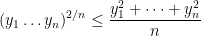
I have just uploaded to the arXiv my paper “A Maclaurin type inequality“. This paper concerns a variant of the Maclaurin inequality for the elementary symmetric means

of real numbers . This inequality asserts that

whenever and are non-negative. It can be proven as a consequence of the Newton inequality

valid for all and arbitrary real (in particular, here the are allowed to be negative). Note that the case of this inequality is just the arithmetic mean-geometric mean inequality

the general case of this inequality can be deduced from this special case by a number of standard manipulations (the most non-obvious of which is the operation of differentiating the real-rooted polynomial to obtain another real-rooted polynomial, thanks to Rolle’s theorem; the key point is that this operation preserves all the elementary symmetric means up to ). One can think of Maclaurin’s inequality as providing a refined version of the arithmetic mean-geometric mean inequality on variables (which corresponds to the case , ).

Whereas Newton’s inequality works for arbitrary real , the Maclaurin inequality breaks down once one or more of the are permitted to be negative. A key example occurs when is even, half of the are equal to , and half are equal to . Here, one can verify that the elementary symmetric means vanish for odd and are equal to for even . In particular, some routine estimation then gives the order of magnitude bound

for even, thus giving a significant violation of the Maclaurin inequality even after putting absolute values around the . In particular, vanishing of one does not imply vanishing of all subsequent .

On the other hand, it was observed by Gopalan and Yehudayoff that if two consecutive values are small, then this makes all subsequent values small as well. More precise versions of this statement were subsequently observed by Meka-Reingold-Tal and Doron-Hatami-Hoza, who obtained estimates of the shape

whenever and are real (but possibly negative). For instance, setting we obtain the inequality

which can be established by combining the arithmetic mean-geometric mean inequality

with the Newton identity

As with the proof of the Newton inequalities, the general case of (2) can be obtained from this special case after some standard manipulations (including the differentiation operation mentioned previously).

However, if one inspects the bound (2) against the bounds (1) given by the key example, we see a mismatch – the right-hand side of (2) is larger than the left-hand side by a factor of about . The main result of the paper rectifies this by establishing the optimal (up to constants) improvement

of (2). This answers a question posed on MathOverflow.

Unlike the previous arguments, we do not rely primarily on the arithmetic mean-geometric mean inequality. Instead, our primary tool is a new inequality

valid for all and . Roughly speaking, the bound (3) would follow from (4) by setting , provided that we can show that the terms of the left-hand side dominate the sum in this regime. This can be done, after a technical step of passing to tuples which nearly optimize the required inequality (3).

We sketch the proof of the inequality (4) as follows. One can use some standard manipulations reduce to the case where and , and after replacing with one is now left with establishing the inequality

Note that equality is attained in the previously discussed example with half of the equal to and the other half equal to , thanks to the binomial theorem.

To prove this identity, we consider the polynomial

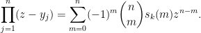
Evaluating this polynomial at , taking absolute values, using the triangle inequality, and then taking logarithms, we conclude that

A convexity argument gives the lower bound

while the normalization gives

and the claim follows.

Undecidability of translational monotilings

Rachel Greenfeld and I have just uploaded to the arXiv our paper “Undecidability of translational monotilings“. This is a sequel to our previous paper in which we constructed a translational monotiling of a high-dimensional lattice (thus the monotile is a finite set and the translates , of partition ) which was aperiodic (there is no way to “repair” this tiling into a periodic tiling , in which is now periodic with respect to a finite index subgroup of ). This disproved the periodic tiling conjecture of Stein, Grunbaum-Shephard and Lagarias-Wang, which asserted that such aperiodic translational monotilings do not exist. (Compare with the “hat monotile“, which is a recently discovered aperiodic isometric monotile for of , where one is now allowed to use rotations and reflections as well as translations, or the even more recent “spectre monotile“, which is similar except that no reflections are needed.)

One of the motivations of this conjecture was the observation of Hao Wang that if the periodic tiling conjecture were true, then the translational monotiling problem is (algorithmically) decidable: there is a Turing machine which, when given a dimension and a finite subset of , can determine in finite time whether can tile . This is because if a periodic tiling exists, it can be found by computer search; and if no tiling exists at all, then (by the compactness theorem) there exists some finite subset of that cannot be covered by disjoint translates of , and this can also be discovered by computer search. The periodic tiling conjecture asserts that these are the only two possible scenarios, thus giving the decidability.

On the other hand, Wang’s argument is not known to be reversible: the failure of the periodic tiling conjecture does not automatically imply the undecidability of the translational monotiling problem, as it does not rule out the existence of some other algorithm to determine tiling that does not rely on the existence of a periodic tiling. (For instance, even with the newly discovered hat and spectre tiles, it remains an open question whether the isometric monotiling problem for (say) polygons with rational coefficients in is decidable, with or without reflections.)

The main result of this paper settles this question (with one caveat):

Theorem 1 There does not exist any algorithm which, given a dimension , a periodic subset of , and a finite subset of , determines in finite time whether there is a translational tiling of by .

The caveat is that we have to work with periodic subsets of , rather than all of ; we believe this is largely a technical restriction of our method, and it is likely that can be removed with additional effort and creativity. We also remark that when , the periodic tiling conjecture was established by Bhattacharya, and so the problem is decidable in the case. It remains open whether the tiling problem is decidable for any fixed value of (note in the above result that the dimension is not fixed, but is part of the input).

Because of a well known link between algorithmic undecidability and logical undecidability (also known as logical independence), the main theorem also implies the existence of an (in principle explicitly describable) dimension , periodic subset of , and a finite subset of , such that the assertion that tiles by translation cannot be proven or disproven in ZFC set theory (assuming of course that this theory is consistent).

As a consequence of our method, we can also replace here by “virtually two-dimensional” groups , with a finite abelian group (which now becomes part of the input, in place of the dimension ).

We now describe some of the main ideas of the proof. It is a common technique to show that a given problem is undecidable by demonstrating that some other problem that was already known to be undecidable can be “encoded” within the original problem, so that any algorithm for deciding the original problem would also decide the embedded problem. Accordingly, we will encode the Wang tiling problem as a monotiling problem in :

Problem 2 (Wang tiling problem) Given a finite collection of Wang tiles (unit squares with each side assigned some color from a finite palette), is it possible to tile the plane with translates of these tiles along the standard lattice , such that adjacent tiles have matching colors along their common edge?

It is a famous result of Berger that this problem is undecidable. The embedding of this problem into the higher-dimensional translational monotiling problem proceeds through some intermediate problems. Firstly, it is an easy matter to embed the Wang tiling problem into a similar problem which we call the domino problem:

Problem 3 (Domino problem) Given a finite collection (resp. ) of horizontal (resp. vertical) dominoes – pairs of adjacent unit squares, each of which is decorated with an element of a finite set of “pips”, is it possible to assign a pip to each unit square in the standard lattice tiling of , such that every horizontal (resp. vertical) pair of squares in this tiling is decorated using a domino from (resp. )?

Indeed, one just has to interpet each Wang tile as a separate “pip”, and define the domino sets , to be the pairs of horizontally or vertically adjacent Wang tiles with matching colors along their edge.

Next, we embed the domino problem into a Sudoku problem:

Problem 4 (Sudoku problem) Given a column width , a digit set , a collection of functions , and an “initial condition” (which we will not detail here, as it is a little technical), is it possible to assign a digit to each cell in the “Sudoku board” such that for any slope and intercept , the digits along the line lie in (and also that obeys the initial condition )?

The most novel part of the paper is the demonstration that the domino problem can indeed be embedded into the Sudoku problem. The embedding of the Sudoku problem into the monotiling problem follows from a modification of the methods in our previous papers, which had also introduced versions of the Sudoku problem, and created a “tiling language” which could be used to “program” various problems, including the Sudoku problem, as monotiling problems.

To encode the domino problem into the Sudoku problem, we need to take a domino function (obeying the domino constraints associated to some domino sets ) and use it to build a Sudoku function (obeying some Sudoku constraints relating to the domino sets); conversely, every Sudoku function obeying the rules of our Sudoku puzzle has to arise somehow from a domino function. The route to doing so was not immediately obvious, but after a helpful tip from Emmanuel Jeandel, we were able to adapt some ideas of Aanderaa and Lewis, in which certain hierarchical structures were used to encode one problem in another. Here, we interpret hierarchical structure -adically (using two different primes due to the two-dimensionality of the domino problem). The Sudoku function that will exemplify our embedding is then built from by the formula

where are two large distinct primes (for instance one can take , for concreteness), denotes the number of times divides , and is the last non-zero digit in the base expansion of :

(with the conventions and ). In the case , the first component of (1) looks like this:

and a typical instance of the final component looks like this:

Amusingly, the decoration here is essentially following the rules of the children’s game “Fizz buzz“.

To demonstrate the embedding, we thus need to produce a specific Sudoku rule (as well as a more technical initial condition , which is basically required to exclude degenerate Sudoku solutions such as a constant solution) that can “capture” the target function (1), in the sense that the only solutions to this specific Sudoku puzzle are given by variants of (e.g., composed with various linear transformations). In our previous paper we were able to build a Sudoku puzzle that could similarly capture either of the first two components , of our target function (1) (up to linear transformations), by a procedure very akin to solving an actual Sudoku puzzle (combined with iterative use of a “Tetris” move in which we eliminate rows of the puzzle that we have fully solved, to focus on the remaining unsolved rows). Our previous paper treated the case when was replaced with a power of , as this was the only case that we know how to embed in a monotiling problem of the entirety of (as opposed to a periodic subset of ), but the analysis is in fact easier when is a large odd prime, instead of a power of . Once the first two components have been solved for, it is a relatively routine matter to design an additional constraint in the Sudoku rule that then constrains the third component to be of the desired form , with obeying the domino constraints.

Monotone non-decreasing sequences of the Euler totient function

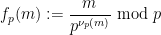
I have just uploaded to the arXiv my paper “Monotone non-decreasing sequences of the Euler totient function“. This paper concerns the quantity , defined as the length of the longest subsequence of the numbers from to for which the Euler totient function is non-decreasing. The first few values of are

(OEIS A365339). For instance, because the totient function is non-decreasing on the set or , but not on the set .

Since for any prime , we have , where is the prime counting function. Empirically, the primes come quite close to achieving the maximum length ; indeed it was conjectured by Pollack, Pomerance, and Treviño, based on numerical evidence, that one had

for all ; this conjecture is verified up to . The previous best known upper bound was basically of the form

as for an explicit constant , from combining results from the above paper with that of Ford or of Maier-Pomerance. In this paper we obtain the asymptotic

so in particular . This answers a question of Erdős, as well as a closely related question of Pollack, Pomerance, and Treviño.

The methods of proof turn out to be mostly elementary (the most advanced result from analytic number theory we need is the prime number theorem with classical error term). The basic idea is to isolate one key prime factor of a given number which has a sizeable influence on the totient function . For instance, for “typical” numbers , one has a factorization

where is a medium sized prime, is a significantly larger prime, and is a number with all prime factors less than . This leads to an approximation

As a consequence, if we temporarily hold fixed, and also localize to a relatively short interval, then can only be non-decreasing in if is also non-decreasing at the same time. This turns out to significantly cut down on the possible length of a non-decreasing sequence in this regime, particularly if is large; this can be formalized by partitioning the range of into various subintervals and inspecting how this (and the monotonicity hypothesis on ) constrains the values of associated to each subinterval. When is small, we instead use a factorization

where is very smooth (i.e., has no large prime factors), and is a large prime. Now we have the approximation

and we can conclude that will have to basically be piecewise constant in order for to be non-decreasing. Pursuing this analysis more carefully (in particular controlling the size of various exceptional sets in which the above analysis breaks down), we end up achieving the main theorem so long as we can prove the preliminary inequality

for all positive rational numbers . This is in fact also a necessary condition; any failure of this inequality can be easily converted to a counterexample to the bound (2), by considering numbers of the form (3) with equal to a fixed constant (and omitting a few rare values of where the approximation (4) is bad enough that is temporarily decreasing). Fortunately, there is a minor miracle, relating to the fact that the largest prime factor of denominator of in lowest terms necessarily equals the largest prime factor of , that allows one to evaluate the left-hand side of (5) almost exactly (this expression either vanishes, or is the product of for some primes ranging up to the largest prime factor of ) that allows one to easily establish (5). If one were to try to prove an analogue of our main result for the sum-of-divisors function , one would need the analogue

of (5), which looks within reach of current methods (and was even claimed without proof by Erdos), but does not have a full proof in the literature at present.

In the final section of the paper we discuss some near counterexamples to the strong conjecture (1) that indicate that it is likely going to be difficult to get close to proving this conjecture without assuming some rather strong hypotheses. Firstly, we show that failure of Legendre’s conjecture on the existence of a prime between any two consecutive squares can lead to a counterexample to (1). Secondly, we show that failure of the Dickson-Hardy-Littlewood conjecture can lead to a separate (and more dramatic) failure of (1), in which the primes are no longer the dominant sequence on which the totient function is non-decreasing, but rather the numbers which are a power of two times a prime become the dominant sequence. This suggests that any significant improvement to (2) would require assuming something comparable to the prime tuples conjecture, and perhaps also some unproven hypotheses on prime gaps.

A lower bound on the mean value of the Erdős-Hooley delta function

Kevin Ford, Dimitris Koukoulopoulos and I have just uploaded to the arXiv our paper “A lower bound on the mean value of the Erdős-Hooley delta function“. This paper complements the recent paper of Dimitris and myself obtaining the upper bound

on the mean value of the Erdős-Hooley delta function

In this paper we obtain a lower bound

where is an exponent that arose in previous work of result of Ford, Green, and Koukoulopoulos, who showed that

for all outside of a set of density zero. The previous best known lower bound for the mean value was

due to Hall and Tenenbaum.

The point is the main contributions to the mean value of are driven not by “typical” numbers of some size , but rather of numbers that have a splitting

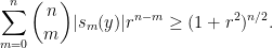
where is the product of primes between some intermediate threshold and and behaves “typically” (so in particular, it has about prime factors, as per the Hardy-Ramanujan law and the Erdős-Kac law, but is the product of primes up to and has double the number of typical prime factors – , rather than – thus is the type of number that would make a significant contribution to the mean value of the divisor function . Here is such that is an integer in the range

for some small constant there are basically different values of give essentially disjoint contributions. From the easy inequalities

(the latter coming from the pigeonhole principle) and the fact that has mean about one, one would expect to get the above result provided that one could get a lower bound of the form

for most typical with prime factors between and . Unfortunately, due to the lack of small prime factors in , the arguments of Ford, Green, Koukoulopoulos that give (1) for typical do not quite work for the rougher numbers . However, it turns out that one can get around this problem by replacing (2) by the more efficient inequality

where

is an enlarged version of when . This inequality is easily proven by applying the pigeonhole principle to the factors of of the form , where is one of the factors of , and is one of the factors of in the optimal interval . The extra room provided by the enlargement of the range to turns out to be sufficient to adapt the Ford-Green-Koukoulopoulos argument to the rough setting. In fact we are able to use the main technical estimate from that paper as a “black box”, namely that if one considers a random subset of for some small and sufficiently large with each lying in with an independent probability , then with high probability there should be subset sums of that attain the same value. (Initially, what “high probability” means is just “close to “, but one can reduce the failure probability significantly as by a “tensor power trick” taking advantage of Bennett’s inequality.)

The convergence of an alternating series of Erdős, assuming the Hardy–Littlewood prime tuples conjecture

I have just uploaded to the arXiv my paper “The convergence of an alternating series of Erdős, assuming the Hardy–Littlewood prime tuples conjecture“. This paper concerns an old problem of Erdős concerning whether the alternating series converges, where denotes the prime. The main result of this paper is that the answer to this question is affirmative assuming a sufficiently strong version of the Hardy–Littlewood prime tuples conjecture.

The alternating series test does not apply here because the ratios are not monotonically decreasing. The deviations of monotonicity arise from fluctuations in the prime gaps , so the enemy arises from biases in the prime gaps for odd and even . By changing variables from to (or more precisely, to integers in the range between and ), this is basically equivalent to biases in the parity of the prime counting function. Indeed, it is an unpublished observation of Said that the convergence of is equivalent to the convergence of . So this question is really about trying to get a sufficiently strong amount of equidistribution for the parity of .

The prime tuples conjecture does not directly say much about the value of ; however, it can be used to control differences for and not too large. Indeed, it is a famous calculation of Gallagher that for fixed , and chosen randomly from to , the quantity is distributed according to the Poisson distribution of mean asymptotically if the prime tuples conjecture holds. In particular, the parity of this quantity should have mean asymptotic to . An application of the van der Corput -process then gives some decay on the mean of as well. Unfortunately, this decay is a bit too weak for this problem; even if one uses the most quantitative version of Gallagher’s calculation, worked out in a recent paper of (Vivian) Kuperberg, the best bound on the mean is something like , which is not quite strong enough to overcome the doubly logarithmic divergence of .

To get around this obstacle, we take advantage of the random sifted model of the primes that was introduced in a paper of Banks, Ford, and myself. To model the primes in an interval such as with drawn randomly from say , we remove one random residue class from this interval for all primes up to Pólya’s “magic cutoff” . The prime tuples conjecture can then be intepreted as the assertion that the random set produced by this sieving process is statistically a good model for the primes in . After some standard manipulations (using a version of the Bonferroni inequalities, as well as some upper bounds of Kuperberg), the problem then boils down to getting sufficiently strong estimates for the expected parity of the random sifted set .

For this problem, the main advantage of working with the random sifted model, rather than with the primes or the singular series arising from the prime tuples conjecture, is that the sifted model can be studied iteratively from the partially sifted sets arising from sifting primes up to some intermediate threshold , and that the expected parity of the experiences some decay in . Indeed, once exceeds the length of the interval , sifting by an additional prime will cause to lose one element with probability , and remain unchanged with probability . If concentrates around some value , this suggests that the expected parity will decay by a factor of about as one increases to , and iterating this should give good bounds on the final expected parity . It turns out that existing second moment calculations of Montgomery and Soundararajan suffice to obtain enough concentration to make this strategy work.

Adjoint Brascamp-Lieb inequalities

Jon Bennett and I have just uploaded to the arXiv our paper “Adjoint Brascamp-Lieb inequalities“. In this paper, we observe that the family of multilinear inequalities known as the Brascamp-Lieb inequalities (or Holder-Brascamp-Lieb inequalities) admit an adjoint formulation, and explore the theory of these adjoint inequalities and some of their consequences.

To motivate matters let us review the classical theory of adjoints for linear operators. If one has a bounded linear operator for some measure spaces and exponents , then one can define an adjoint linear operator involving the dual exponents , obeying (formally at least) the duality relation

for suitable test functions on respectively. Using the dual characterization

of (and similarly for ), one can show that has the same operator norm as .

There is a slightly different way to proceed using Hölder’s inequality. For sake of exposition let us make the simplifying assumption that (and hence also ) maps non-negative functions to non-negative functions, and ignore issues of convergence or division by zero in the formal calculations below. Then for any reasonable function on , we have

by (1) and Hölder; dividing out by we obtain , and a similar argument also recovers the reverse inequality.

The first argument also extends to some extent to multilinear operators. For instance if one has a bounded bilinear operator for then one can then define adjoint bilinear operators and obeying the relations

and with exactly the same operator norm as . It is also possible, formally at least, to adapt the Hölder inequality argument to reach the same conclusion.

In this paper we observe that the Hölder inequality argument can be modified in the case of Brascamp-Lieb inequalities to obtain a different type of adjoint inequality. (Continuous) Brascamp-Lieb inequalities take the form

for various exponents and surjective linear maps , where are arbitrary non-negative measurable functions and is the best constant for which this inequality holds for all such . [There is also another inequality involving variances with respect to log-concave distributions that is also due to Brascamp and Lieb, but it is not related to the inequalities discussed here.] Well known examples of such inequalities include Hölder’s inequality and the sharp Young convolution inequality; another is the Loomis-Whitney inequality, the first non-trivial example of which is

for all non-negative measurable . There are also discrete analogues of these inequalities, in which the Euclidean spaces are replaced by discrete abelian groups, and the surjective linear maps are replaced by discrete homomorphisms.

The operation of pulling back a function on by a linear map to create a function on has an adjoint pushforward map , which takes a function on and basically integrates it on the fibers of to obtain a “marginal distribution” on (possibly multiplied by a normalizing determinant factor). The adjoint Brascamp-Lieb inequalities that we obtain take the form

for non-negative and various exponents , where is the optimal constant for which the above inequality holds for all such ; informally, such inequalities control the norm of a non-negative function in terms of its marginals. It turns out that every Brascamp-Lieb inequality generates a family of adjoint Brascamp-Lieb inequalities (with the exponent being less than or equal to ). For instance, the adjoints of the Loomis-Whitney inequality (2) are the inequalities

for all non-negative measurable , all summing to , and all , where the exponents are defined by the formula

and the are the marginals of :

One can derive these adjoint Brascamp-Lieb inequalities from their forward counterparts by a version of the Hölder inequality argument mentioned previously, in conjunction with the observation that the pushforward maps are mass-preserving (i.e., they preserve the norm on non-negative functions). Conversely, it turns out that the adjoint Brascamp-Lieb inequalities are only available when the forward Brascamp-Lieb inequalities are. In the discrete case the forward and adjoint Brascamp-Lieb constants are essentially identical, but in the continuous case they can (and often do) differ by up to a constant. Furthermore, whereas in the forward case there is a famous theorem of Lieb that asserts that the Brascamp-Lieb constants can be computed by optimizing over gaussian inputs, the same statement is only true up to constants in the adjoint case, and in fact in most cases the gaussians will fail to optimize the adjoint inequality. The situation appears to be complicated; roughly speaking, the adjoint inequalities only use a portion of the range of possible inputs of the forward Brascamp-Lieb inequality, and this portion often misses the gaussian inputs that would otherwise optimize the inequality.

We have located a modest number of applications of the adjoint Brascamp-Lieb inequality (but hope that there will be more in the future):

• The inequalities become equalities at ; taking a derivative at this value (in the spirit of the replica trick in physics) we recover the entropic Brascamp-Lieb inequalities of Carlen and Cordero-Erausquin. For instance, the derivative of the adjoint Loomis-Whitney inequalities at yields Shearer’s inequality.
• The adjoint Loomis-Whitney inequalities, together with a few more applications of Hölder’s inequality, implies the log-concavity of the Gowers uniformity norms on non-negative functions, which was previously observed by Shkredov and by Manners.
• Averaging the adjoint Loomis-Whitney inequalities over coordinate systems gives reverse inequalities for the X-ray transform and other tomographic transforms that appear to be new in the literature. In particular, we obtain some monotonicity of the norms or entropies of the -plane transform in (if the exponents are chosen in a dimensionally consistent fashion).

We also record a number of variants of the adjoint Brascamp-Lieb inequalities, including discrete variants, and a reverse inequality involving norms with rather than .

Sumsets and entropy revisited

Ben Green, Freddie Manners and I have just uploaded to the arXiv our preprint “Sumsets and entropy revisited“. This paper uses entropy methods to attack the Polynomial Freiman-Ruzsa (PFR) conjecture, which we study in the following two forms:

Conjecture 1 (Weak PFR over ) Let be a finite non-empty set whose doubling constant is at most . Then there is a subset of of density that has affine dimension (i.e., it is contained in an affine space of dimension ).

Conjecture 2 (PFR over ) Let be a non-empty set whose doubling constant is at most . Then can be covered by cosets of a subspace of cardinality at most .

Our main results are then as follows.

Theorem 3 If with , then

• (i) There is a subset of of density of “skew-dimension” (or “query complexity”) .
• (ii) There is a subset of of density of affine dimension (where goes to zero as ).
• (iii) If Conjecture 2 holds, then there is a subset of of density of affine dimension . In other words, Conjecture 2 implies Conjecture 1.

The skew-dimension of a set is a quantity smaller than the affine dimension which is defined recursively; the precise definition is given in the paper, but suffice to say that singleton sets have dimension , and a set whose projection to has skew-dimension at most , and whose fibers in have skew-dimension at most for any , will have skew-dimension at most . (In fact, the skew-dimension is basically the largest quantity which obeys all of these properties.)

Part (i) of this theorem was implicitly proven by Pálvölgi and Zhelezov by a different method. Part (ii) with replaced by was established by Manners. To our knowledge, part (iii) is completely new.

Our proof strategy is to establish these combinatorial additive combinatorics results by using entropic additive combinatorics, in which we replace sets with random variables , and cardinality with (the exponential of) Shannon entropy. This is in order to take advantage of some superior features of entropic additive combinatorics, most notably good behavior with respect to homomorphisms.

For instance, the analogue of the combinatorial doubling constant of a finite non-empty subset of an abelian group , is the entropy doubling constant

of a finitely-valued random variable in , where are independent copies of and denotes Shannon entropy. There is also an analogue of the Ruzsa distance

between two finite non-empty subsets of , namely the entropic Ruzsa distance

where are independent copies of respectively. (Actually, one thing we show in our paper is that the independence hypothesis can be dropped, and this only affects the entropic Ruzsa distance by a factor of three at worst.) Many of the results about sumsets and Ruzsa distance have entropic analogues, but the entropic versions are slightly better behaved; for instance, we have a contraction property

whenever is a homomorphism. In fact we have a refinement of this inequality in which the gap between these two quantities can be used to control the entropic distance between “fibers” of (in which one conditions and to be fixed). On the other hand, there are direct connections between the combinatorial and entropic sumset quantities. For instance, if is a random variable drawn uniformly from , then

Thus if has small doubling, then has small entropic doubling. In the converse direction, if has small entropic doubling, then is close (in entropic Ruzsa distance) to a uniform random variable drawn from a set of small doubling; a version of this statement was proven in an old paper of myself, but we establish here a quantitatively efficient version, established by rewriting the entropic Ruzsa distance in terms of certain Kullback-Liebler divergences.

Our first main result is a “99% inverse theorem” for entropic Ruzsa distance: if is sufficiently small, then there exists a finite subgroup of such that

This result uses the results just mentioned to relate to a set of small doubling, which can then be related to a subgroup by standard inverse theorems; this gives a weak version of (1) (roughly speaking losing a square root in the bound), and some additional analysis is needed to bootstrap this initial estimate back to (1).

We now sketch how these tools are used to prove our main theorem. For (i), we reduce matters to establishing the following bilinear entropic analogue: given two non-empty finite subsets of , one can find subsets , with

such that have skew-dimension at most , for some absolute constant . This can be shown by an induction on (say). One applies a non-trivial coordinate projection to . If and are very close in entropic Ruzsa distance, then the 99% inverse theorem shows that these random variables must each concentrate at a point (because has no non-trivial finite subgroups), and can pass to a fiber of these points and use the induction hypothesis. If instead and are far apart, then by the behavior of entropy under projections one can show that the fibers of and under are closer on average in entropic Ruzsa distance of and themselves, and one can again proceed using the induction hypothesis.

For parts (ii) and (iii), we first use an entropic version of an observation of Manners that sets of small doubling in must be irregularly distributed modulo . A clean formulation of this in entropic language is the inequality

whenever take values in a torsion-free abelian group such as ; this turns out to follow from two applications of the entropy submodularity inequality. One corollary of this (and the behavior of entropy under projections) is that

This is the key link between the and worlds that is used to prove (ii), (iii): while (iii) relies on the still unproven PFR conjecture over , (ii) uses the unconditional progress on PFR by Konyagin, as detailed in this survey of Sanders. The argument has a similar inductive structure to that used to establish (i) (and if one is willing to replace by then the argument is in fact relatively straightforward and does not need any deep partial results on the PFR).

As one byproduct of our analysis we also obtain an appealing entropic reformulation of Conjecture 2, namely that if is an -valued random variable then there exists a subspace of such that

Right now the best result in this direction is

for any , by using Konyagin’s partial result towards the PFR.