
You are currently browsing the tag archive for the ‘divisor function’ tag.
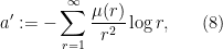
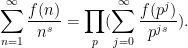
Kaisa Matomäki, Xuancheng Shao, Joni Teräväinen, and myself have just uploaded to the arXiv our preprint “Higher uniformity of arithmetic functions in short intervals I. All intervals“. This paper investigates the higher order (Gowers) uniformity of standard arithmetic functions in analytic number theory (and specifically, the Möbius function 


![{(X,X+H]}](https://s0.wp.com/latex.php?latex=%7B%28X%2CX%2BH%5D%7D&bg=ffffff&fg=000000&s=0&c=20201002)


 , where
  . For applications in the additive combinatorics of such functions , it is also necessary to consider more general correlations, such as polynomial correlations
 is a polynomial of some fixed degree, or more generally
 is a nilmanifold of fixed degree and dimension (and with some control on structure constants),
  is a polynomial map, and
  is a Lipschitz function (with some bound on the Lipschitz constant). Indeed, thanks to the inverse theorem for the Gowers uniformity norm, such correlations let one control the Gowers uniformity norm of (possibly after subtracting off some renormalising factor) on such short intervals , which can in turn be used to control other multilinear correlations involving such functions.
Traditionally, asymptotics for such sums are expressed in terms of a “main term” of some arithmetic nature, plus an error term that is estimated in magnitude. For instance, a sum such as 

 variable to be restricted further to a subprogression of , but let us ignore this minor extension for this discussion). There is some flexibility in how to choose these approximants, but we eventually found it convenient to use the following choices.
- For the Möbius function
, as per the Möbius pseudorandomness conjecture. (One could choose a more sophisticated approximant in the presence of a Siegel zero, as I did with Joni in this recent paper, but we do not do so here.)
- For the von Mangoldt function
, where
and
.
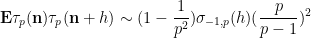
- For the divisor functions
for some explicit polynomials
, chosen so that
and
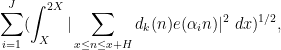
The objective is then to obtain bounds on sums such as (1) that improve upon the “trivial bound” that one can get with the triangle inequality and standard number theory bounds such as the Brun-Titchmarsh inequality. For 


Our main estimates on sums of the form (1) work in the following ranges:
- For
, one can obtain strongly logarithmic savings on (1) for
, and power savings for
.
- For
, one can obtain weakly logarithmic savings for
.
- For
, one can obtain power savings for
.
- For
, one can obtain power savings for
.
Conjecturally, one should be able to obtain power savings in all cases, and lower 

By combining these results with tools from additive combinatorics, one can obtain a number of applications:
- Direct insertion of our bounds in the recent work of Kanigowski, Lemanczyk, and Radziwill on the prime number theorem on dynamical systems that are analytic skew products gives some improvements in the exponents there.
- We can obtain a “short interval” version of a multiple ergodic theorem along primes established by Frantzikinakis-Host-Kra and Wooley-Ziegler, in which we average over intervals of the form
.
- We can obtain a “short interval” version of the “linear equations in primes” asymptotics obtained by Ben Green, Tamar Ziegler, and myself in this sequence of papers, where the variables in these equations lie in short intervals
We now briefly discuss some of the ingredients of proof of our main results. The first step is standard, using combinatorial decompositions (based on the Heath-Brown identity and (for the 
- Type
sums, which are basically of the form
for some weights
of controlled size and some cutoff
that is not too large;
- Type
sums, which are basically of the form
for some weights
of controlled size and some cutoffs
that are not too close to
or to
- Type
sums, which are basically of the form
for some weights
The precise ranges of the cutoffs 
The Type
For the Type 


 range in various dyadic intervals. Using the known multidimensional equidistribution theory of polynomial maps in nilmanifolds, one can eventually show in the non-abelian case that this sequence either has enough equidistribution to give cancellation, or else the nilsequence involved can be replaced with one from a lower dimensional nilmanifold, in which case one can apply an induction hypothesis.
For the type

 into a number of arithmetic progressions, and then uses equidistribution theory to establish cancellation of sequences such as
  on the majority of these progressions. As it turns out, this strategy works well in the regime
  unless the nilsequence involved is “major arc”, but the latter case is treatable by existing methods as discussed previously; this is why the exponent for our
  result can be as low as
  .
.
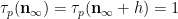
In a sequel to this paper (currently in preparation), we will obtain analogous results for almost all intervals ![{(x,x+H]}](https://s0.wp.com/latex.php?latex=%7B%28x%2Cx%2BH%5D%7D&bg=ffffff&fg=000000&s=0&c=20201002)

![{[X,2X]}](https://s0.wp.com/latex.php?latex=%7B%5BX%2C2X%5D%7D&bg=ffffff&fg=000000&s=0&c=20201002)

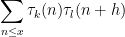
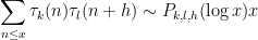
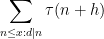
Kaisa Matomaki, Maksym Radziwill, and I have uploaded to the arXiv our paper “Correlations of the von Mangoldt and higher divisor functions II. Divisor correlations in short ranges“. This is a sequel of sorts to our previous paper on divisor correlations, though the proof techniques in this paper are rather different. As with the previous paper, our interest is in correlations such as

for medium-sized 


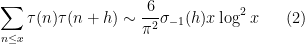
As discussed in this previous post, one heuristically expects an asymptotic of the form

for any fixed 


for 


for 


We now discuss some of the ingredients of the proof. Unsurprisingly, the first step is the circle method, expressing (1) in terms of exponential sums such as

Actually, it is convenient to first prune 

In our previous paper on bounded multiplicative functions, we used Plancherel’s theorem to estimate the global 


for a moderate number of disjoint intervals 


where 


after various averaging in the 

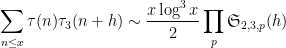
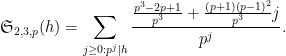
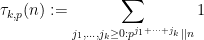
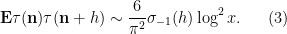
This is a postscript to the previous blog post which was concerned with obtaining heuristic asymptotic predictions for the correlation

for the divisor function 
when
for fixed 
is the order 


or more accurately
where 


for some polynomial 


In principle, the calculations of the previous post should recover the predictions of Conrey and Gonek. In this post I would like to record this for the top order term:
Conjecture 1 If
and
are fixed, then
as
, where the product is over all primes
, and the local factors
are given by the formula
where
is the degree
polynomial
where
and one adopts the conventions that
and
for
.


For instance, if

and hence
and the above conjecture recovers the Ingham formula (2). For 

and so we predict
where
Similarly, if 


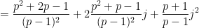
and so we predict

where

and so forth.
As in the previous blog, the idea is to factorise
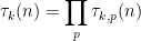
where the local factors 
(where 


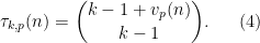
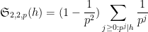
We then have the following exact local asymptotics:
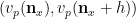
Proposition 2 (Local correlations) Let
be a profinite integer chosen uniformly at random, let


(For profinite integers it is possible that 

Conjecture 1 can then be heuristically justified from the local calculations (2) by various pseudorandomness heuristics, as discussed in the previous post.
I’ll give a short proof of the above proposition below, basically using the recursive methods of the previous post. This short proof actually took be quite a while to find; I spent several hours and a fair bit of scratch paper working out the cases 

It was only after expending all this effort that I realised that it would be much more efficient to compute the correlations for all values of 
I am confident that Conjecture 1 is consistent with the explicit asymptotic in the Conrey-Gonek conjecture, but have not yet rigorously established that the leading order term in the latter is indeed identical to the expression provided above.
Let
where 


that is to say the random variable 


Now we turn to the pair correlations 

The error term in (2) has been refined by many subsequent authors, as has the uniformity of the estimates in the
Using our probabilistic lens, the estimate (2) can be written as
From (1) (and the asymptotic negligibility of the shift by 


Ingham’s formula can be established in a number of ways. Firstly, one can expand out 


for various 


Each of the methods outlined above requires a fair amount of calculation, and it is not obvious while performing them that the factor 


using symmetry to order 


and we obtain the desired consistency after multiplying by
This still however does not explain the presence of the 
One heuristic way to proceed is through analysis of local factors. Observe from the fundamental theorem of arithmetic that we can factor
where the product is over all primes 


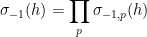
where
(or in terms of valuations, 


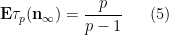
Proposition 1 (Local Ingham asymptotics) For fixed
and
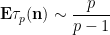

From the Euler formula

we see that
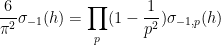
and so one can “explain” the arithmetic factor 
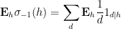
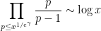
Remark 2 The relation between the local means
and the global mean
can also be seen heuristically through the application
of Mertens’ theorem, where
is Pólya’s magic exponent, which serves as a useful heuristic limiting threshold in situations where the product of local factors is divergent.
Let us now prove this proposition. One could brute-force the computations by observing that for any fixed 

It is first convenient to get rid of error terms by observing that in the limit 


in the profinite setting (this setting will make it easier to set up the recursion).
We begin with (5). Observe that 


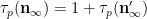
As 

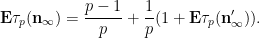
We use a similar method to treat (6). First treat the case when 


and the claim (6) in this case follows from (5) and a brief computation (noting that 
Now suppose that 


which by (5) (and replacing

and (6) then follows by induction on the number of powers of
The estimate (2) of Ingham was refined by Estermann, who obtained the more accurate expansion


for certain complicated but explicit coefficients 

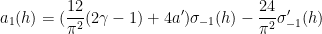
where 
The formula for 


These lower order terms are traditionally computed either from a Dirichlet series approach (using Perron’s formula) or a circle method approach. It turns out that a refinement of the above heuristics can also predict these lower order terms, thus keeping the calculation purely in physical space as opposed to the “multiplicative frequency space” of the Dirichlet series approach, or the “additive frequency space” of the circle method, although the computations are arguably as messy as the latter computations for the purposes of working out the lower order terms. We illustrate this just for the 
In analytic number theory, an arithmetic function is simply a function 


whenever 


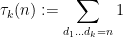
that counts the number of divisors of a natural number 

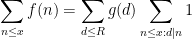
There are various approaches to multiplicative number theory, each of which focuses on different asymptotic statistics of arithmetic functions
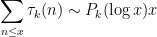
- The summatory functions
of an arithmetic function
(if it exists).
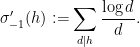
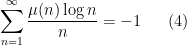
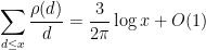
- The logarithmic sums
of an arithmetic function
(if it exists).


Here, we are normalising the arithmetic function 

A classical case of interest is when 

Typically, the logarithmic sums are relatively easy to control, but the summatory functions require more effort in order to obtain satisfactory estimates; see Exercise 6 below.
If an arithmetic function
for various real or complex numbers 


In the elementary approach to multiplicative number theory presented in this set of notes, we consider Dirichlet series only for real numbers 
Remark 1 The elementary and complex-analytic approaches to multiplicative number theory are the two classical approaches to the subject. One could also consider a more “Fourier-analytic” approach, in which one studies convolution-type statistics such as
as
for various cutoff functions
, such as smooth, compactly supported functions. See this previous blog post for an instance of such an approach. Another related approach is the “pretentious” approach to multiplicative number theory currently being developed by Granville-Soundararajan and their collaborators. We will occasionally make reference to these more modern approaches in these notes, but will primarily focus on the classical approaches.
To reverse the process and derive control on summatory functions or logarithmic sums starting from control of Dirichlet series is trickier, and usually requires one to allow
The basic strategy of elementary multiplicative theory is to first gather useful estimates on the statistics of “smooth” or “non-oscillatory” functions, such as the constant function 


This is only an introduction to elementary multiplicative number theory techniques. More in-depth treatments may be found in this text of Montgomery-Vaughan, or this text of Bateman-Diamond.
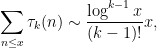
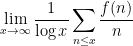
One of the basic problems in analytic number theory is to obtain bounds and asymptotics for sums of the form

in the limit 
where

It is thus of interest to develop techniques to estimate such sums 
At the easiest end of the spectrum are those functions 


One can already get quite good bounds on this quantity by comparison with the integral 

with sharper bounds available by using tools such as the Euler-Maclaurin formula (see this blog post). Exponentiating such asymptotics, incidentally, leads to one of the standard proofs of Stirling’s formula (as discussed in this blog post).
One can also consider “non-Archimedean” notions of smoothness, such as periodicity relative to a small period 


In particular, we have the fundamental estimate

This is a good estimate when 

One can also consider functions

where
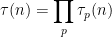
Another class of functions that is reasonably well controlled are the multiplicative functions, in which 


which are clearly related to the partial sums
One also obtains similar types of representations for functions that are not quite multiplicative, but are closely related to multiplicative functions, such as the von Mangoldt function 
Moving another notch along the spectrum between well-controlled and ill-controlled functions, one can consider functions

for some other arithmetic function 


and thus by (1) one can bound this by the sum of a main term 

or expressions of the form

where each 
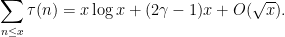
One of the simplest examples of this comes when estimating the divisor function

which counts the number of divisors up to


Here, we are (barely) able to keep the error term smaller than the main term; this is right at the edge of the divisor sum method, because the level

where 


From Dirichlet series methods, it is not difficult to establish the identities
and

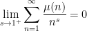
This suggests (but does not quite prove) that one has

in the sense of conditionally convergent series. Assuming one can justify this (which, ultimately, requires one to exclude zeroes of the Riemann zeta function on the line 


However, there are a number of tricks available to reduce the level of divisor sums. The simplest comes from exploiting the change of variables 


except when
This type of argument is also known as the Dirichlet hyperbola method. A variant of this argument can also deduce the prime number theorem from (3), (4) (and with some additional effort, one can even drop the use of (4)); this is discussed at this previous blog post.
Using this square root trick, one can now also control divisor sums such as

(Note that 


which one can rewrite as

The constraint 

where 


The function 


and also

and thus

Similar arguments give asymptotics for 


However, the square root trick is insufficient by itself to deal with higher order sums involving the divisor function, such as

the level here is initially of order 

Nevertheless, there is an ingenious argument of Erdös that allows one to obtain good upper and lower bounds for these sorts of sums, in particular establishing the asymptotic
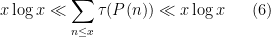
for any fixed irreducible non-constant polynomial 


for any fixed 


for any fixed
The lower bound in (6) is easy, since one can simply lower the level in (5) to obtain the lower bound

for any 

for any fixed 


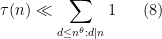
This however can be fixed in a number of ways. First of all, even when 

for some 

For Erdös’s upper bound (6), though, one cannot afford to lose these additional factors of 


which, thanks to Mertens’ theorem
for some absolute constant 


The Erdös argument is quite robust; for instance, the more general inequality

for fixed irreducible

which turn out to be enough to obtain the right asymptotics for the number of solutions to the equation 
Below the fold I will provide some more details of the arguments of Landreau and of Erdös.
Given a positive integer 


then (by the fundamental theorem of arithmetic)

Clearly, 

for any 


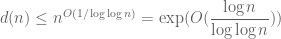
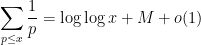
The divisor bound is useful in many applications in number theory, harmonic analysis, and even PDE (on periodic domains); it asserts that for any large number n, only a “logarithmically small” set of numbers less than n will actually divide n exactly, even in the worst-case scenario when n is smooth. (The average value of d(n) is much smaller, being about 

or from the heuristic that a randomly chosen number m less than n has a probability about 1/m of dividing n, and 
The divisor bound is elementary to prove (and not particularly difficult), and I was asked about it recently, so I thought I would provide the proof here, as it serves as a case study in how to establish worst-case estimates in elementary multiplicative number theory.
[Update, Sep 24: some applications added.]

Recent Comments