
You are currently browsing the category archive for the ‘math.CV’ category.
Previous set of notes: Notes 3. Next set of notes: 246C Notes 1.
One of the great classical triumphs of complex analysis was in providing the first complete proof (by Hadamard and de la Vallée Poussin in 1896) of arguably the most important theorem in analytic number theory, the prime number theorem:
Theorem 1 (Prime number theorem) Letdenote the number of primes less than a given real number
. Then
(or in asymptotic notation,
as
).
(Actually, it turns out to be slightly more natural to replace the approximation 

The complex-analytic proof of this theorem hinges on the study of a key meromorphic function related to the prime numbers, the Riemann zeta function 
Definition 2 (Riemann zeta function, preliminary definition) Letbe such that
. Then we define

Note that the series is locally uniformly convergent in the half-plane
The Riemann zeta function has several remarkable properties, some of which we summarise here:
Theorem 3 (Basic properties of the Riemann zeta function)
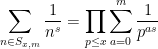
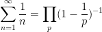
- (i) (Euler product formula) For any
where the product is absolutely convergent (and locally uniform in
) and is over the prime numbers
.
- (ii) (Trivial zero-free region)
has no zeroes in the region
.
- (iii) (Meromorphic continuation)
and no other poles. Furthermore, the Riemann xi function
is an entire function of order
(after removing all singularities). The function
is an entire function of order one after removing the singularity at
- (iv) (Functional equation) After applying the meromorphic continuation from (iii), we have
for all
for all


Proof: We just prove (i) and (ii) for now, leaving (iii) and (iv) for later sections.
The claim (i) is an encoding of the fundamental theorem of arithmetic, which asserts that every natural number 


 ,
,  , and
, and  consists of all the natural numbers of the form
  for some
  . Sending
  and to infinity, we conclude from monotone convergence and the geometric series formula that
 is real, and then from dominated convergence we see that the same formula holds for complex with as well. Local uniform convergence then follows from the product form of the Weierstrass
  -test (Exercise 19 of Notes 1).
The claim (ii) is immediate from (i) since the Euler product 

We remark that by sending
 . This can be viewed as a weak version of the prime number theorem, and already illustrates the potential applicability of the Riemann zeta function to control the distribution of the prime numbers.
The meromorphic continuation (iii) of the zeta function is initially surprising, but can be interpreted either as a manifestation of the extremely regular spacing of the natural numbers 
Henceforth we work with the meromorphic continuation of 


From Theorem 3 and the non-vanishing nature of 


 by (1), hence for all (except the pole at ) by meromorphic continuation. Thus if is a non-trivial zero then so is
  . We conclude that the set of non-trivial zeroes is symmetric by reflection by both the real axis and the critical line
  . We have the following infamous conjecture:
Conjecture 4 (Riemann hypothesis) All the non-trivial zeroes of
This conjecture would have many implications in analytic number theory, particularly with regard to the distribution of the primes. Of course, it is far from proven at present, but the partial results we have towards this conjecture are still sufficient to establish results such as the prime number theorem.
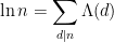
Return now to the original region where


 , where the von Mangoldt function
  is defined to equal
  whenever
  is a power
  of a prime
  for some
  , and
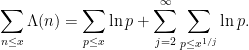
, and  otherwise. The contribution of the higher prime powers
  is negligible in practice, and as a first approximation one can think of the von Mangoldt function as the indicator function of the primes, weighted by the logarithm function.
The series 

Exercise 5 (Standard Dirichlet series) Let
- (i) Show that
.
- (ii) Show that
, where
is the divisor function of
- (iii) Show that
, where
is the Möbius function, defined to equal
when
distinct primes for some
, and
otherwise.
- (iv) Show that
, where
is the Liouville function, defined to equal
- (v) Show that
, where
is the holomorphic branch of the logarithm that is real for
vanishes for
.
- (vi) Use the fundamental theorem of arithmetic to show that the von Mangoldt function is the unique function
such that
for every positive integer
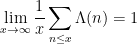
Given the appearance of the von Mangoldt function 
Theorem 6 (Prime number theorem, von Mangoldt form) One has(or in asymptotic notation,
as
Let us see how Theorem 6 implies Theorem 1. Firstly, for any 
 is non-zero for only
  values of
  , and is of size
  , thus
 , we conclude from Theorem 6 that
  . Next, observe from the fundamental theorem of calculus that
 and summing over all primes
  , we conclude that
 , thus
 and
and  we see that the right-hand side is
  , and Theorem 1 follows.
Exercise 7 Show that Theorem 1 conversely implies Theorem 6.
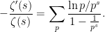
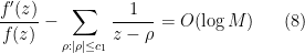
The alternate form (8) of the Euler product identity connects the primes (represented here via proxy by the von Mangoldt function) with the logarithmic derivative of the zeta function, and can be used as a starting point for describing further relationships between
Theorem 8 (Riemann-von Mangoldt explicit formula) For any non-integer, we have
where
. Furthermore, the convergence of the limit is locally uniform in

Actually, it turns out that this formula is in some sense too precise; in applications it is often more convenient to work with smoothed variants of this formula in which the sum on the left-hand side is smoothed out, but the contribution of zeroes with large imaginary part is damped; see Exercise 22. Nevertheless, this formula clearly illustrates how the non-trivial zeroes

 )
) 
 induces an oscillation in the von Mangoldt function, with
  controlling the frequency of the oscillation and
  the rate to which the oscillation dies out as
  . This relationship is sometimes known informally as “the music of the primes”.
Comparing Theorem 8 with Theorem 6, it is natural to suspect that the key step in the proof of the latter is to establish the following slight but important extension of Theorem 3(ii), which can be viewed as a very small step towards the Riemann hypothesis:
Theorem 9 (Slight enlargement of zero-free region) There are no zeroes of.
It is not quite immediate to see how Theorem 6 follows from Theorem 8 and Theorem 9, but we will demonstrate it below the fold.
Although Theorem 9 only seems like a slight improvement of Theorem 3(ii), proving it is surprisingly non-trivial. The basic idea is the following: if there was a zero at 


 can be negative for large regions of the variable , whereas is always non-negative. This conflict eventually leads to a contradiction, but it is not immediately obvious how to make this argument rigorous. We will present here the classical approach to doing so using a trigonometric identity of Mertens.
In fact, Theorem 9 is basically equivalent to the prime number theorem:
Exercise 10 For the purposes of this exercise, assume Theorem 6, but do not assume Theorem 9. For any non-zero realas
, where
denotes a quantity that goes to zero as
. Use this to derive Theorem 9.

This equivalence can help explain why the prime number theorem is remarkably non-trivial to prove, and why the Riemann zeta function has to be either explicitly or implicitly involved in the proof.
This post is only intended as the briefest of introduction to complex-analytic methods in analytic number theory; also, we have not chosen the shortest route to the prime number theorem, electing instead to travel in directions that particularly showcase the complex-analytic results introduced in this course. For some further discussion see this previous set of lecture notes, particularly Notes 2 and Supplement 3 (with much of the material in this post drawn from the latter).
Previous set of notes: Notes 2. Next set of notes: Notes 4.
On the real line, the quintessential examples of a periodic function are the (normalised) sine and cosine functions 

 and we obtain more general trigonometric polynomials that are -periodic; and the theory of Fourier series tells us that all other -periodic functions (with reasonable integrability conditions) can be approximated in various senses by such polynomial combinations. Using Euler’s identity, one can use
  and
and  in place of and as the basic generating functions here, provided of course one is willing to use complex coefficients instead of real ones. Of course, by rescaling one can also make similar statements for other periods than . -periodic functions
  can also be identified (by abuse of notation) with functions
  on the quotient space
  (known as the additive -torus or additive unit circle), or with functions
 ![{f: [0,1] \rightarrow {\bf C}}](https://s0.wp.com/latex.php?latex=%7Bf%3A+%5B0%2C1%5D+%5Crightarrow+%7B%5Cbf+C%7D%7D&bg=ffffff&fg=000000&s=0&c=20201002) on the fundamental domain (up to boundary)
on the fundamental domain (up to boundary) ![{[0,1]}](https://s0.wp.com/latex.php?latex=%7B%5B0%2C1%5D%7D&bg=ffffff&fg=000000&s=0&c=20201002) of that quotient space with the periodic boundary condition
of that quotient space with the periodic boundary condition  . The map
  also identifies the additive unit circle with the geometric unit circle
  , thanks in large part to the fundamental trigonometric identity
  ; this can also be identified with the multiplicative unit circle
  . (Usually by abuse of notation we refer to all of these three sets simultaneously as the “unit circle”.) Trigonometric polynomials on the additive unit circle then correspond to ordinary polynomials of the real coefficients
  of the geometric unit circle, or Laurent polynomials of the complex variable
  .
.
What about periodic functions on the complex plane? We can start with singly periodic functions 


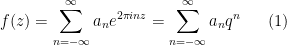
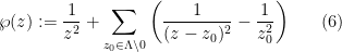
Proposition 1 (Description of singly periodic holomorphic functions)In both cases, the coefficients
- (i) Every
where
is the nome
, and the
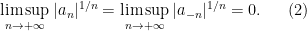
are complex coefficients such that
Conversely, every doubly infinite sequence
of coefficients obeying (2) gives rise to a
- (ii) Every bounded
on the upper half-plane
has an expansion
where the
Conversely, every infinite sequence
for every
).
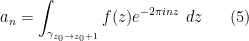
by the Fourier inversion formula
for any
in
(in case (i)) or
(in case (ii)).


Proof: If 


For part (ii), we observe that the map 


The additive cylinder 

Now let us turn attention to doubly periodic functions of a complex variable

 and some periods
  , which to avoid degeneracies we will assume to be linearly independent over the reals (thus
  are non-zero and the ratio
  is not real). One can rescale by a common scaling factor
  to normalise either
  or
or  , but one of course cannot simultaneously normalise both parameters in this fashion. As in the singly periodic case, such functions can also be identified with functions on the additive
  -torus
  , where is the lattice
  , or with functions on the solid parallelogram bounded by the contour
  (a fundamental domain up to boundary for that torus), obeying the boundary periodicity conditions
  in the edge
  , and
, and  in the edge
  .
.
Within the world of holomorphic functions, the collection of doubly periodic functions is boring:
Proposition 2 Let). Then
In the language of Riemann surfaces, this proposition asserts that the torus
Proof: The fundamental domain (up to boundary) enclosed by 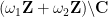
To obtain more interesting examples of doubly periodic functions, one must therefore turn to the world of meromorphic functions – or equivalently, holomorphic functions into the Riemann sphere 
 for -periodic real functions. This function will have a double pole at the origin , and more generally at all other points on the lattice , but no other poles. The derivative
  , and plays a role analogous to
  . Remarkably, all the other doubly periodic meromorphic functions with these periods will turn out to be rational combinations of
  and
and  ; furthermore, in analogy with the identity
  , one has an identity of the form
  (avoiding poles) and some complex numbers
  that depend on the lattice . Indeed, much as the map
  creates a diffeomorphism between the additive unit circle to the geometric unit circle
  , the map
  turns out to be a complex diffeomorphism between the torus and the elliptic curve
 maps the origin
  of the torus to the point
  at infinity. (Indeed, one can view elliptic curves as “multiplicative tori”, and both the additive and multiplicative tori can be identified as smooth manifolds with the more familiar geometric torus, but we will not use such an identification here.) This fundamental identification with elliptic curves and tori motivates many of the further remarkable properties of elliptic curves; for instance, the fact that tori are obviously an abelian group gives rise to an abelian group law on elliptic curves (and this law can be interpreted as an analogue of the trigonometric sum identities for
  ). The description of the various meromorphic functions on the torus also helps motivate the more general Riemann-Roch theorem that is a fundamental law governing meromorphic functions on other compact Riemann surfaces (and is discussed further in these 246C notes). So far we have focused on studying a single torus . However, another important mathematical object of study is the space of all such tori, modulo isomorphism; this is a basic example of a moduli space, known as the (classical, level one) modular curve
  . This curve can be described in a number of ways. On the one hand, it can be viewed as the upper half-plane
  quotiented out by the discrete group
  ; on the other hand, by using the -invariant, it can be identified with the complex plane ; alternatively, one can compactify the modular curve and identify this compactification with the Riemann sphere . (This identification, by the way, produces a very short proof of the little and great Picard theorems, which we proved in 246A Notes 4.) Functions on the modular curve (such as the -invariant) can be viewed as -invariant functions on , and include the important class of modular functions; they naturally generalise to the larger class of (weakly) modular forms, which are functions on which transform in a very specific way under -action, and which are ubiquitous throughout mathematics, and particularly in number theory. Basic examples of modular forms include the Eisenstein series, which are also the Laurent coefficients of the Weierstrass elliptic functions . More number theoretic examples of modular forms include (suitable powers of) theta functions , and the modular discriminant
  . Modular forms are -periodic functions on the half-plane, and hence by Proposition 1 come with Fourier coefficients ; these coefficients often turn out to encode a surprising amount of number-theoretic information; a dramatic example of this is the famous modularity theorem, (a special case of which was) used amongst other things to establish Fermat’s last theorem. Modular forms can be generalised to other discrete groups than (such as congruence groups) and to other domains than the half-plane , leading to the important larger class of automorphic forms, which are of major importance in number theory and representation theory, but which are well outside the scope of this course to discuss.
Previous set of notes: Notes 1. Next set of notes: Notes 3.
In Exercise 5 (and Lemma 1) of 246A Notes 4 we already observed some links between complex analysis on the disk (or annulus) and Fourier series on the unit circle:
- (i) Functions
are expressed by a convergent Fourier series (and also Taylor series)
for
(so in particular
), where
conversely, every infinite sequenceof coefficients obeying (1) arises from such a function
- (ii) Functions
are expressed by a convergent Fourier series (and also Laurent series)
, where
conversely, every doubly infinite sequenceof coefficients obeying (2) arises from such a function
- (iii) In the situation of (ii), there is a unique decomposition
where
extends holomorphically to
, and
extends holomorphically to
and goes to zero at infinity, and are given by the formulae
where
where


This connection lets us interpret various facts about Fourier series through the lens of complex analysis, at least for some special classes of Fourier series. For instance, the Fourier inversion formula 


It turns out that there are similar links between complex analysis on a half-plane (or strip) and Fourier integrals on the real line, which we will explore in these notes.
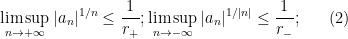
We first fix a normalisation for the Fourier transform. If 


Exercise 1 (Fourier transform of Gaussian) Ifis a complex number with
and
, show that the Fourier transform
, where we use the standard branch for
.
The Fourier transform has many remarkable properties. On the one hand, as long as the function

Exercise 2 (Decay ofHint: to establish holomorphicity in each of these cases, use Morera’s theorem and the Fubini-Tonelli theorem. For uniqueness, use analytic continuation, or (for part (iv)) the Schwartz reflection principle.
- (i) If
for all
and
(that is to say one has
for some finite quantity
depending only on
), then
. Furthermore, this function continues to be defined by (3).
- (ii) If
then the entire function
for
. In particular, if
then
.
- (iii) If
for all
, then
, and obeys the bound
in this strip. Furthermore, this function continues to be defined by (3).
- (iv) If
(resp.
), then there is a unique continuous extension of
(resp. the upper half-plane
) which is holomorphic in the interior of this half-plane, and such that
uniformly as
(resp.
). Furthermore, this function continues to be defined by (3).
Later in these notes we will give a partial converse to part (ii) of this exercise, known as the Paley-Wiener theorem; there are also partial converses to the other parts of this exercise.
From (3) we observe the following intertwining property between multiplication by an exponential and complex translation: if 

The material in these notes is loosely adapted from Chapter 4 of Stein-Shakarchi’s “Complex Analysis”.
Previous set of notes: 246A Notes 5. Next set of notes: Notes 2.
— 1. Jensen’s formula —
Suppose 
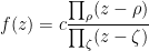
 , where ranges over the zeroes of
  (counting multiplicity) and ranges over the zeroes of
  (counting multiplicity), and assuming avoids the zeroes of . Taking absolute values and then logarithms, we arrive at the formula
  avoids the zeroes of both and . (In this set of notes we use
  for the natural logarithm when applied to a positive real number, and
  for the standard branch of the complex logarithm (which extends ); the multi-valued complex logarithm will only be used in passing.) Alternatively, taking logarithmic derivatives, we arrive at the closely related formula
  avoiding the zeroes of both and . Thus we see that the zeroes and poles of a rational function describe the behaviour of that rational function, as well as close relatives of that function such as the log-magnitude
  and log-derivative
  . We have already seen these sorts of formulae arise in our treatment of the argument principle in 246A Notes 4.
Exercise 1 Letbe a complex polynomial of degree
.
- (i) (Gauss-Lucas theorem) Show that the complex roots of
are contained in the closed convex hull of the complex roots of
- (ii) (Laguerre separation theorem) If all the complex roots of
, and
, then all the complex roots of
are also contained in
There are a number of useful ways to extend these formulae to more general meromorphic functions than rational functions. Firstly there is a very handy “local” variant of (1) known as Jensen’s formula:
Theorem 2 (Jensen’s formula) Let, with all removable singularities removed. Then, if
where
.

One can view (3) as a truncated (or localised) variant of (1). Note also that the summands 
Proof: By perturbing 


 has no zeroes or poles inside the disk, it has a holomorphic logarithm (Exercise 46 of 246A Notes 4). In particular,
  is the real part of . The claim now follows by applying the mean value property (Exercise 17 of 246A Notes 3) to .
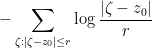
An important special case of Jensen’s formula arises when 
Exercise 3 Use (6) to give another proof of Liouville’s theorem: a bounded holomorphic function
Exercise 4 Use Jensen’s formula to prove the fundamental theorem of algebra: a complex polynomialfor some complex numbers
with
. (Note that the fundamental theorem was invoked previously in this section, but only for motivational purposes, so the proof here is non-circular.)
Exercise 5 (Shifted Jensen’s formula) Let, with all removable singularities removed. Show that
for all
that are not zeroes or poles of
and
. (The function
appearing in the integrand is sometimes known as the Poisson kernel, particularly if one normalises so that


Exercise 6 (Bounded type)
- (i) If
.
- (ii) If
. (Functions
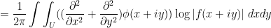
Exercise 7 (Smoothed out Jensen formula) Let, and let
be a smooth compactly supported function. Show that
where
range over the zeroes and poles of
. Informally argue why this identity is consistent with Jensen’s formula. (Note: as many of the functions involved here are not holomorphic, complex analysis tools are of limited use. Try using real variable tools such as Stokes theorem, Greens theorem, or integration by parts.)
When applied to entire functions
Proposition 8 Letfor some
and all
such that
has at most
zeroes (counting multiplicity) for any
.
Entire functions that obey a growth bound of the form 


Proof: First suppose that 

 contribute at least
  to a summand on the right-hand side, while all other zeroes contribute a non-negative quantity, thus
 denotes the number of zeroes in . This gives the claim for
  . When
  , one can shift by a small amount to make non-zero at the origin (using the fact that zeroes of holomorphic functions not identically zero are isolated), modifying
  in the process, and then repeating the previous arguments.
Just as (3) and (7) give truncated variants of (1), we can create truncated versions of (2). The following crude truncation is adequate for many applications:
Theorem 9 (Truncated formula for log-derivative) Letfor some
and all
. Let
be constants. Then one has the approximate formula
for all
other than zeroes of
.
Proof: To abbreviate notation, we allow all implied constants in this proof to depend on 
We mimic the proof of Jensen’s formula. Firstly, we may translate and rescale so that 


 is
is  , as claimed.
Suppose 


 and is
  , and hence
  for . Thus we see from (9) that we may use Blaschke products to remove all the zeroes in the annulus while only affecting the left-hand side of (8) by
  ; also, removing the Blaschke products does not affect
  on the unit circle, and only affects
  by thanks to (9). Thus we may assume without loss of generality that there are no zeroes in this annulus.
Similarly, given a zero 

![{t \in [0,1]}](https://s0.wp.com/latex.php?latex=%7Bt+%5Cin+%5B0%2C1%5D%7D&bg=ffffff&fg=000000&s=0&c=20201002)

 for any real )

 and its first derivatives are
  on the disk
  . But recall from the proof of Jensen’s formula that is the derivative of a logarithm
  of , whose real part is . By the Cauchy-Riemann equations for , we conclude that
  on the disk , as required.
Exercise 10
- (i) (Borel-Carathéodory theorem) If
is analytic on an open neighborhood of a disk
and
, show that
(Hint: one can normalise
,
. Now
. Use a Möbius transformation to map the half-plane to the unit disk and then use the Schwarz lemma.)
- (ii) Use (i) to give an alternate way to conclude the proof of Theorem 9.

A variant of the above argument allows one to make precise the heuristic that holomorphic functions locally look like polynomials:
Exercise 11 (Local Weierstrass factorisation) Let the notation and hypotheses be as in Theorem 9. Then show thatfor all
(counting multiplicity) and
is a holomorphic function on
and first derivative
on this disk. Furthermore, show that the degree of

Exercise 12 (Preliminary Beurling factorisation) Letdenote the space of bounded analytic functions
on the unit disk; this is a normed vector space with norm
- (i) If
is not identically zero, and
denote the zeroes of
and
- (ii) Let the notation be as in (i). If we define the Blaschke product
where
for all
. (It may be easier to work with finite Blaschke products first to obtain this bound.)
- (iii) Continuing the notation from (i), establish a factorisation
for some holomorphic function
with
for all
.
- (iv) (Theorem of F. and M. Riesz, special case) If
, show that the set
has zero measure.


Remark 13 The factorisation (iii) can be refined further, with. There are also extensions to larger spaces
than
is to
), known as Hardy spaces. We will not discuss this topic further here, but see for instance this text of Garnett for a treatment.
Exercise 14 (Littlewood’s lemma) Letfor some
and
, with
where
which is continuous on the upper, lower, and right edges of


Just a short announcement that next quarter I will be continuing the recently concluded 246A complex analysis class as 246B. Topics I plan to cover:
- Schwartz-Christoffel transformations and the uniformisation theorem (using the remainder of the 246A notes);
- Jensen’s formula and factorisation theorems (particularly Weierstrass and Hadamard); the Gamma function;
- Connections with the Fourier transform on the real line;
- Elliptic functions and their relatives;
- (if time permits) the Riemann zeta function and the prime number theorem.
Notes for the later material will appear on this blog in due course.
I’ve just uploaded to the arXiv my paper “Sendov’s conjecture for sufficiently high degree polynomials“. This paper is a contribution to an old conjecture of Sendov on the zeroes of polynomials:
Conjecture 1 (Sendov’s conjecture) Letthat has all zeroes in the closed unit disk
. If
is one of these zeroes, then
has at least one zero in
.
It is common in the literature on this problem to normalise
Many cases of this conjecture are already known, for instance
- When
(Brown-Xiang 1999);
- When
(Gauss-Lucas theorem);
- When
(Bojanov 2011);
- When
for a fixed
, and
- When
for a sufficiently large absolute constant
- When
(Rubinstein 1968; Goodman-Rahman-Ratti 1969; Joyal 1969);
- When
, where
is sufficiently small depending on
- When
(Chijiwa 2011);
- When
(Kasmalkar 2014).
In particular, in high degrees the only cases left uncovered by prior results are when
Our main result covers the high degree case uniformly for all values of ![{a \in [0,1]}](https://s0.wp.com/latex.php?latex=%7Ba+%5Cin+%5B0%2C1%5D%7D&bg=ffffff&fg=000000&s=0&c=20201002)
Theorem 2 There exists an absolute constantsuch that Sendov’s conjecture holds for all
.
In principle, this reduces the verification of Sendov’s conjecture to a finite time computation, although our arguments use compactness methods and thus do not easily provide an explicit value of 
Because of the previous results (particularly those of Chalebgwa and Chijiwa), we will only need to establish the following two subcases of the above theorem:
Theorem 3 (Sendov’s conjecture near the origin) Under the additional hypothesis, Sendov’s conjecture holds for sufficiently large
Theorem 4 (Sendov’s conjecture near the unit circle) Under the additional hypothesisfor a fixed
, Sendov’s conjecture holds for sufficiently large
We approach these theorems using the “compactness and contradiction” strategy, assuming that there is a sequence of counterexamples whose degrees
I also found it useful to use the language of probability theory. Given a putative counterexample 

 are linked to each other by the identity
 inside the unit disk
  . Applying Prokhorov’s theorem, and passing to a subsequence, one can then assume that the random variables converge in distribution to some limiting random variables
  (possibly defined on a different probability space than the original variables ), also living almost surely inside the unit disk. Standard potential theory then gives the convergence

 sense. Among other things, we then conclude from the identity (2) and some elementary inequalities that
 . This turns out to have an appealing interpretation in terms of Brownian motion: if one takes two Brownian motions in the complex plane, one originating from
  and one originating from
  , then the location where these Brownian motions first exit the unit disk will have the same distribution. (In our paper we actually replace Brownian motion with the closely related formalism of balayage.) This turns out to connect the random variables , quite closely to each other. In particular, with this observation and some additional arguments involving both the unique continuation property for harmonic functions and Grace’s theorem (discussed in this previous post), with the latter drawn from the prior work of Dégot, we can get very good control on these distributions:
Theorem 5
- (i) If
, then
and have the same distribution.
- (ii) If
, then
, and
In case (i) (and strengthening the hypothesis 


Case (ii) turns out to be more delicate. This is because there are a number of “near-counterexamples” to Sendov’s conjecture that are compatible with the hypotheses and conclusion of case (ii). The simplest such example is 


 for some constants
  and
and  , one eventually would be able to arrive at a true counterexample to Sendov’s conjecture if these locations
  were in the open lune
 . However, if one takes the mean of this inequality in , one arrives at the inequality
 and
and  . In order to extend this argument to more general polynomials , we require a stability analysis of the endpoint equation
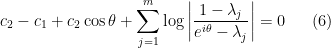
 and
and  . The above discussion then places all the zeros
  on the arc
 vanish), because all the non-zero elements of the arc (7) have argument in
 ![{\pm [\pi/3,\pi/2]}](https://s0.wp.com/latex.php?latex=%7B%5Cpm+%5B%5Cpi%2F3%2C%5Cpi%2F2%5D%7D&bg=ffffff&fg=000000&s=0&c=20201002) , so in particular their square
, so in particular their square  will have negative real part. It turns out that one can adapt this argument to the more general potential counterexamples to Sendov’s conjecture (in the form of Theorem 4). The starting point is to use (1), (4), and Theorem 5(ii) to obtain good control on
  , which one then integrates and exponentiates to get good control on , and then on a second integration one gets enough information about to pin down the location of its zeroes to high accuracy. The constraint that these zeroes lie inside the unit disk then gives an inequality resembling (5), and an adaptation of the above stability analysis is then enough to conclude. The arguments here are inspired by the previous arguments of Miller, which treated the case when was extremely close to via a similar perturbative analysis; the main novelty is to control the error terms not in terms of the magnitude of the largest zero of (which is difficult to manage when gets large), but rather by the variance of those zeroes, which ends up being a more tractable expression to keep track of.
Consider a disk 


Theorem 1 (Holomorphic images of disks) Letbe a holomorphic function with
.
- (i) (Open mapping theorem or inverse function theorem)
contains a disk
for some
to
- (ii) (Bloch theorem)
for some absolute constant
. (In fact there is even a holomorphic right inverse of
- (iii) (Koebe quarter theorem) If
.
- (iv) If
.
- (v) If one has a bound of the form
for all
and some
, then
for some absolute constant
Parts (i), (ii), (iii) of this theorem are standard, as indicated by the given links. I found part (iv) as (a consequence of) Theorem 2 of this paper of Degot, who remarks that it “seems not already known in spite of its simplicity”; an equivalent form of this result also appears in Lemma 4 of this paper of Miller. The proof is simple:
Proof: (Proof of (iv)) Let 


 ). But by the fundamental theorem of algebra we have
 are the roots of the polynomial (counting multiplicity). By the pigeonhole principle, there must therefore exist a root
  of
of  such that
 . Thus contains
  , and the claim follows.
The constant 


 . This example also shows that despite parts (ii), (iii) of the theorem, one cannot hope for a general inclusion of the form
  .
.
Part (v) is implicit in the standard proof of Bloch’s theorem (part (ii)), and is easy to establish:
Proof: (Proof of (v)) From the Cauchy inequalities one has 


Note that part (v) implies part (i). A standard point picking argument also lets one deduce part (ii) from part (v):
Proof: (Proof of (ii)) By shrinking 


 such that
  . Iterating this procedure in the obvious fashion we either are done, or obtain a Cauchy sequence
  in such that
  goes to infinity as
  , which contradicts the analytic nature of (and hence continuous nature of ) on the closure of . This gives the claim.
Here is another classical result stated by Alexander (and then proven by Kakeya and by Szego, but also implied to a classical theorem of Grace and Heawood) that is broadly compatible with parts (iii), (iv) of the above theorem:
Proposition 2 Letfor all
.
The radius 


If one narrows 


To recover the best constant of
Proposition 3 (Grace-Heawood theorem) Let. Then
.
This is in turn implied by a remarkable and powerful theorem of Grace (which we shall prove shortly). Given two polynomials 


Theorem 4 (Grace’s theorem) Letinto two open connected regions
. Let
and all the zeroes of
. Then
.
(Contrapositively: if 
Indeed, a brief calculation reveals the identity
 is the degree
  polynomial
  are
are  for
for  , so the Grace-Heawood theorem follows by applying Grace’s theorem with equal to the boundary of
  .
.
The same method of proof gives the following nice consequence:
Theorem 5 (Perpendicular bisector theorem) Letbe a polynomial such that
. Then the zeroes of
or the halfplane
.
I’d be interested in seeing a proof of this latter theorem that did not proceed via Grace’s theorem.
Now we give a proof of Grace’s theorem. The case 


 , it suffices to establish the skew-adjointness relation
Next, we see that the inversion map 


 , with each Möbius transformation
  mapping each to
  , where
  is the unique (up to constants) rational function that maps this a map from to (its divisor is
  ). Since the Möbius transformations are generated by translations and inversion, we see that the action of Möbius transformations projectively preserves the apolar form; also, we see this action of
  on also moves the zeroes of each by (viewing polynomials of degree less than in as having zeroes at infinity). In particular, the hypotheses and conclusions of Grace’s theorem are preserved by this Möbius action. We can then apply such a transformation to move one of the zeroes of to infinity (thus making a polynomial of degree ), so that must now be a circle, with the zeroes of inside the circle and the remaining zeroes of outside the circle. But then
 are also inside . The claim now follows from the induction hypothesis.
Dimitri Shlyakhtenko and I have uploaded to the arXiv our paper Fractional free convolution powers. For me, this project (which we started during the 2018 IPAM program on quantitative linear algebra) was motivated by a desire to understand the behavior of the minor process applied to a large random Hermitian 


 , and are often arranged in a triangular array known as a Gelfand-Tsetlin pattern, as discussed in these previous blog posts.
When 


As first observed by Bercovici and Voiculescu and developed further by Nica and Speicher, among other authors, the notion of a free convolution power
 , and can be defined by solving the Burgers-type equation
 (see this previous blog post for a derivation). This equation can be solved explicitly using the -transform
  of , defined by solving the equation
  , in which case one can show that
 , the -transform is simply the identity:
  .)
.)
Nica and Speicher also gave a free probability interpretation of the fractional free convolution power: if 


![{[pAp]}](https://s0.wp.com/latex.php?latex=%7B%5BpAp%5D%7D&bg=ffffff&fg=000000&s=0&c=20201002)

![{[pXp]}](https://s0.wp.com/latex.php?latex=%7B%5BpXp%5D%7D&bg=ffffff&fg=000000&s=0&c=20201002)

![{\tau_p([pXp]) := k \tau(pXp)}](https://s0.wp.com/latex.php?latex=%7B%5Ctau_p%28%5BpXp%5D%29+%3A%3D+k+%5Ctau%28pXp%29%7D&bg=ffffff&fg=000000&s=0&c=20201002)
One of the known facts about integer free convolution powers

 is monotone non-decreasing for integer , and the Fisher information
  is monotone non-increasing for integer . This is the free probability analogue of the corresponding monotonicities for differential entropy and classical Fisher information that was established by Artstein, Ball, Barthe, and Naor, answering a question of Shannon.
Our first main result is to extend the monotonicity results of Shylakhtenko to fractional 
 is a polynomial and
  is a semicircular element free of
  . If has an absolutely continuous law
  for a sufficiently regular , one can calculate explicitly as
  , where
  is the Hilbert transform of , and the Fisher information is given by the formula
 relative to some subalgebra
  of noncommutative random variables.
The free score interacts very well with the free minor process ![{X \mapsto [pXp]}](https://s0.wp.com/latex.php?latex=%7BX+%5Cmapsto+%5BpXp%5D%7D&bg=ffffff&fg=000000&s=0&c=20201002)
![\displaystyle J( [pXp] : [pBp] ) = k {\bf E}( [p J(X:B) p] | [pXp], [pBp] )](https://s0.wp.com/latex.php?latex=%5Cdisplaystyle++J%28+%5BpXp%5D+%3A+%5BpBp%5D+%29+%3D+k+%7B%5Cbf+E%7D%28+%5Bp+J%28X%3AB%29+p%5D+%7C+%5BpXp%5D%2C+%5BpBp%5D+%29&bg=ffffff&fg=000000&s=0&c=20201002) is a noncommutative random variable, is an algebra of noncommutative random variables, and is a real projection of trace that is free of both and . The monotonicity of free Fisher information then follows from an application of Pythagoras’s theorem (which implies in particular that conditional expectation operators are contractions on
is a noncommutative random variable, is an algebra of noncommutative random variables, and is a real projection of trace that is free of both and . The monotonicity of free Fisher information then follows from an application of Pythagoras’s theorem (which implies in particular that conditional expectation operators are contractions on  ). The monotonicity of free entropy then follows from an integral representation of free entropy as an integral of free Fisher information along the free Ornstein-Uhlenbeck process (or equivalently, free Fisher information is essentially the rate of change of free entropy with respect to perturbation by semicircular noise). The argument also shows when equality holds in the monotonicity inequalities; this occurs precisely when is a semicircular measure up to affine rescaling.
After an extensive amount of calculation of all the quantities that were implicit in the above free probability argument (in particular computing the various terms involved in the application of Pythagoras’ theorem), we were able to extract a self-contained proof of monotonicity that relied on differentiating the quantities in 

 is the kernel
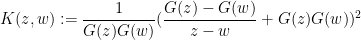
 . It is not difficult to show that
  is a positive semi-definite kernel, which gives the required monotonicity. It would be interesting to obtain some more insightful interpretation of the kernel and the identity (2).
These monotonicity properties hint at the minor process ![{A \mapsto [pAp]}](https://s0.wp.com/latex.php?latex=%7BA+%5Cmapsto+%5BpAp%5D%7D&bg=ffffff&fg=000000&s=0&c=20201002)


![\displaystyle \mu^{\boxplus 1/s}((-\infty,\lambda(s,y)/s])=y/s,](https://s0.wp.com/latex.php?latex=%5Cdisplaystyle++%5Cmu%5E%7B%5Cboxplus+1%2Fs%7D%28%28-%5Cinfty%2C%5Clambda%28s%2Cy%29%2Fs%5D%29%3Dy%2Fs%2C&bg=ffffff&fg=000000&s=0&c=20201002) is sufficiently well behaved. The random matrix interpretation of is that it is the asymptotic location of the
is sufficiently well behaved. The random matrix interpretation of is that it is the asymptotic location of the  eigenvalue of the
  upper left minor of a random matrix with asymptotic empirical spectral distribution and with unitarily invariant distribution, thus is in some sense a continuum limit of Gelfand-Tsetlin patterns. Thus for instance the Cauchy interlacing laws in this asymptotic limit regime become

 is the Lagrangian density
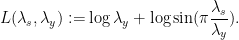
 . The quantity
  measures the mean eigenvalue spacing at some location of the Gelfand-Tsetlin pyramid, and the ratio
  measures mean eigenvalue drift in the minor process. This suggests that this Lagrangian density is some sort of measure of entropy of the asymptotic microscale point process emerging from the minor process at this spacing and drift. There is work of Metcalfe demonstrating that this point process is given by the Boutillier bead model, so we conjecture that this Lagrangian density somehow measures the entropy density of this process.
Kari Astala, Steffen Rohde, Eero Saksman and I have (finally!) uploaded to the arXiv our preprint “Homogenization of iterated singular integrals with applications to random quasiconformal maps“. This project started (and was largely completed) over a decade ago, but for various reasons it was not finalised until very recently. The motivation for this project was to study the behaviour of “random” quasiconformal maps. Recall that a (smooth) quasiconformal map is a homeomorphism

 ; this can be viewed as a deformation of the Cauchy-Riemann equation
  . Assuming that
  is asymptotic to at infinity, one can (formally, at least) solve for in terms of using the Beurling transform
 if
if  is a random field that oscillates at some fine spatial scale
  . A simple model to keep in mind is
 ![\displaystyle \mu_\delta(z) = \varphi(z) \sum_{n \in {\bf Z}^2} \epsilon_n 1_{n\delta + [0,\delta]^2}(z) \ \ \ \ \ (1)](https://s0.wp.com/latex.php?latex=%5Cdisplaystyle++%5Cmu_%5Cdelta%28z%29+%3D+%5Cvarphi%28z%29+%5Csum_%7Bn+%5Cin+%7B%5Cbf+Z%7D%5E2%7D+%5Cepsilon_n+1_%7Bn%5Cdelta+%2B+%5B0%2C%5Cdelta%5D%5E2%7D%28z%29+%5C+%5C+%5C+%5C+%5C+%281%29&bg=ffffff&fg=000000&s=0&c=20201002)
 are independent random signs and
  is a bump function. For models such as these, we show that a homogenisation occurs in the limit
  ; each multilinear expression
 to a lacunary sequence) to a deterministic limit, and the associated quasiconformal map
  similarly converges weakly in probability (or almost surely). (Results of this latter type were also recently obtained by Ivrii and Markovic by a more geometric method which is simpler, but is applied to a narrower class of Beltrami coefficients.) In the specific case (1), the limiting quasiconformal map is just the identity map
  , but if for instance replaces the
  by non-symmetric random variables then one can have significantly more complicated limits. The convergence theorem for multilinear expressions such as is not specific to the Beurling transform ; any other translation and dilation invariant singular integral can be used here.
The random expression (2) is somewhat reminiscent of a moment of a random matrix, and one can start computing it analogously. For instance, if one has a decomposition 

 .
.
If all the 
 collide with each other, preventing one from easily factoring the expression. A typical problematic contribution for instance would be a sum of the form

 in the latter sum, then it splits into
 requires an inclusion-exclusion argument that creates some notational headaches but is ultimately manageable.) As the name suggests, the non-split configurations such as (4) cannot be factored in this fashion, and are the most difficult to handle. A direct computation using the triangle inequality (and a certain amount of combinatorics and induction) reveals that these sums are somewhat localised, in that dyadic portions such as
  (when measured in suitable function space norms), basically because of the large number of times one has to transition back and forth between
  and
and  . Thus, morally at least, the dominant contribution to a non-split sum such as (4) comes from the local portion when
  . From the translation and dilation invariance of this type of expression then simplifies to something like
 , and this can be shown to converge to a weak limit as .
In principle all of these limits are computable, but the combinatorics is remarkably complicated, and while there is certainly some algebraic structure to the calculations, it does not seem to be easily describable in terms of an existing framework (e.g., that of free probability).
A useful rule of thumb in complex analysis is that holomorphic functions
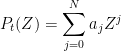
In some cases it can be convenient instead to work with polynomials 


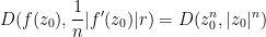
one ends up having the following heuristic approximation in the neighbourhood of a point 
Heuristic 1 (Polynomial approximation) Let
be a height, let
, and let
be an integer. Let
be the linear change of variables
for
and some polynomial
of degree

The requirement 


Let us give two non-rigorous justifications of this heuristic. Firstly, it is standard that inside the critical strip (with 

of (11). If we group the integers 

For 

and so

where 
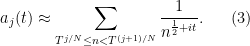
This gives the desired polynomial approximation.
A second non-rigorous justification is as follows. From factorisation theorems such as the Hadamard factorisation theorem we expect to have
where 

again ignoring all issues of convergence. If one writes 
(here we are glossing over some technical issues regarding renormalisation of the infinite products, which can be dealt with by studying the asymptotics as 

This again gives the desired polynomial approximation.
Below the fold we give a rigorous version of the second argument suitable for “microscale” analysis. More precisely, we will show
Theorem 2 Let
be an integer going sufficiently slowly to infinity. Let
go to zero sufficiently slowly depending on
(in the limit
), and possibly after adjusting
of degree
whenever
.

It should be possible to refine the arguments to extend this theorem to the mesoscale setting by letting 


Many conjectures and arguments involving the Riemann zeta function can be heuristically translated into arguments involving the polynomials 


Let’s now heuristically explore the polynomial analogues of this theory in a bit more detail. The Riemann hypothesis basically corresponds to the assertion that all the 


where

A routine calculation involving Stirling’s formula reveals that

with 

when 

 ,
, 
where 
then the functional equation can be written as

We remark that if we use the heuristic (3) (interpreting the cutoffs in the
Another consequence of the functional equation is that the zeroes of 


One consequence of the functional equation is that 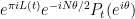


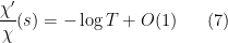
Relating to this fact, it is a classical result of Speiser that the Riemann hypothesis is true if and only if all the zeroes of the derivative
Proposition 3 We have
(where all zeroes are counted with multiplicity.) In particular, the zeroes of
lie in the closed unit disk.

Proof: From the functional equation we have

Thus it will suffice to show that
Set 


(This can also be seen by writing 
From the functional equation and the chain rule, 


One can use this identity to get a lower bound on the number of zeroes of 


By Jensen’s formula, we have for any 


We therefore have

As the logarithm function is concave, we can apply Jensen’s inequality to conclude

where the expectation is over the 


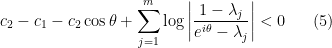
The zeroes of

where 

and the right-hand side is of unit magnitude by the functional equation. However, if we differentiate
where 

The right-hand side would now be typically expected to be of size 


Recent Comments