
You are currently browsing the monthly archive for July 2013.
As in all previous posts in this series, we adopt the following asymptotic notation: 


The purpose of this (rather technical) post is both to roll over the polymath8 research thread from this previous post, and also to record the details of the latest improvement to the Type I estimates (based on exploiting additional averaging and using Deligne’s proof of the Weil conjectures) which lead to a slight improvement in the numerology.
In order to obtain this new Type I estimate, we need to strengthen the previously used properties of “dense divisibility” or “double dense divisibility” as follows.
Definition 1 (Multiple dense divisibility) Let
. For each natural number
, we define a notion of
-tuply
-dense divisibility recursively as follows:
- Every natural number
is
-tuply
- If
and
are natural numbers with
, and
, one can find a factorisation
with
such that
-tuply
is
-tuply
We let
denote the set of
-tuply densely divisible” as “densely divisible”, “
-tuply densely divisible” as “doubly densely divisible”, and so forth; we also abbreviate
as
.
Given any finitely supported sequence 


We now recall the key concept of a coefficient sequence, with some slight tweaks in the definitions that are technically convenient for this post.
Definition 2 A coefficient sequence is a finitely supported sequence
that obeys the bounds
for all
is the divisor function.
- (i) A coefficient sequence
is said to be located at scale
for some
if it is supported on an interval of the form
for some
.
- (ii) A coefficient sequence
for any
, any fixed
, and any primitive residue class
.
- (iii) A coefficient sequence
is said to be smooth if it takes the form
for some smooth function
supported on an interval of size
and obeying the derivative bounds
for all fixed
(note that the implied constant in the
notation may depend on


Note that we allow sequences to be smooth at scale 


Now we adapt the Type I estimate to the
Definition 3 (Type I estimates) Let
,
, and
be fixed quantities, and let
be an arbitrary bounded subset of
, let
, and let
a primitive congruence class. We say that
holds if, whenever
are quantities with
for some fixed
, and
are coefficient sequences located at scales
respectively, with
obeying a Siegel-Walfisz theorem, we have
for any fixed
. Here, as in previous posts,
denotes the square-free natural numbers whose prime factors lie in

The main theorem of this post is then
Theorem 4 (Improved Type I estimate) We have
whenever
and

In practice, the first condition here is dominant. Except for weakening double dense divisibility to quadruple dense divisibility, this improves upon the previous Type I estimate that established ![{Type^{(2)}_I[\varpi,\delta,\sigma]}](https://s0.wp.com/latex.php?latex=%7BType%5E%7B%282%29%7D_I%5B%5Cvarpi%2C%5Cdelta%2C%5Csigma%5D%7D&bg=ffffff&fg=000000&s=0&c=20201002)

As in previous posts, Type I estimates (when combined with existing Type II and Type III estimates) lead to distribution results of Motohashi-Pintz-Zhang type. For any fixed 
![{MPZ^{(k)}[\varpi,\delta]}](https://s0.wp.com/latex.php?latex=%7BMPZ%5E%7B%28k%29%7D%5B%5Cvarpi%2C%5Cdelta%5D%7D&bg=ffffff&fg=000000&s=0&c=20201002)
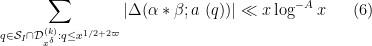
![\displaystyle \sum_{q \in {\mathcal S}_I \cap {\mathcal D}_{x^\delta}^{(k)}: q \leq x^{1/2+2\varpi}} |\Delta(\Lambda 1_{[x,2x]}; a\ (q))| \ll x \log^{-A} x \ \ \ \ \ (7)](https://s0.wp.com/latex.php?latex=%5Cdisplaystyle++%5Csum_%7Bq+%5Cin+%7B%5Cmathcal+S%7D_I+%5Ccap+%7B%5Cmathcal+D%7D_%7Bx%5E%5Cdelta%7D%5E%7B%28k%29%7D%3A+q+%5Cleq+x%5E%7B1%2F2%2B2%5Cvarpi%7D%7D+%7C%5CDelta%28%5CLambda+1_%7B%5Bx%2C2x%5D%7D%3B+a%5C+%28q%29%29%7C+%5Cll+x+%5Clog%5E%7B-A%7D+x+%5C+%5C+%5C+%5C+%5C+%287%29&bg=ffffff&fg=000000&s=0&c=20201002)
for any fixed 

![{MPZ^{(4)}[\varpi,\delta]}](https://s0.wp.com/latex.php?latex=%7BMPZ%5E%7B%284%29%7D%5B%5Cvarpi%2C%5Cdelta%5D%7D&bg=ffffff&fg=000000&s=0&c=20201002) whenever
whenever 
Proof: Setting 

![{Type^{(4)}_{II}[\varpi,\delta]}](https://s0.wp.com/latex.php?latex=%7BType%5E%7B%284%29%7D_%7BII%7D%5B%5Cvarpi%2C%5Cdelta%5D%7D&bg=ffffff&fg=000000&s=0&c=20201002)

and

The second condition is implied by the first and can be deleted.
From this previous post we know that ![{Type'_{II}[\varpi,\delta], Type''_{II}[\varpi,\delta]}](https://s0.wp.com/latex.php?latex=%7BType%27_%7BII%7D%5B%5Cvarpi%2C%5Cdelta%5D%2C+Type%27%27_%7BII%7D%5B%5Cvarpi%2C%5Cdelta%5D%7D&bg=ffffff&fg=000000&s=0&c=20201002)
while ![{Type^{(4)}_{III}[\varpi,\delta,\sigma]}](https://s0.wp.com/latex.php?latex=%7BType%5E%7B%284%29%7D_%7BIII%7D%5B%5Cvarpi%2C%5Cdelta%2C%5Csigma%5D%7D&bg=ffffff&fg=000000&s=0&c=20201002)

Again, these conditions are implied by (8). The claim then follows from the Heath-Brown identity and dyadic decomposition as in this previous post.

As before, we let ![{DHL[k_0,2]}](https://s0.wp.com/latex.php?latex=%7BDHL%5Bk_0%2C2%5D%7D&bg=ffffff&fg=000000&s=0&c=20201002)


 .
.
This follows from the Pintz sieve, as discussed below the fold. Combining this with the best known prime tuples, we obtain that there are infinitely many prime gaps of size at most 

If 


A simple application of the Fubini-Tonelli theorem shows that the convolution 


where 
The convolution

for any bounded measurable function 


for any bounded (Borel) measurable function
for all Borel measurable 


If 


While the above discussion gives a perfectly rigorous definition of the convolution of two measures, it does not always give helpful guidance as to how to compute the convolution of two explicit measures (e.g. the convolution of two surface measures on explicit examples of surfaces, such as the sphere). In simple cases, one can work from first principles directly from the definition (2), (3), perhaps after some application of tools from several variable calculus, such as the change of variables formula. Another technique proceeds by regularisation, approximating the measures 

(where we identify an absolutely integrable function 


A third method proceeds using the Fourier transform
of
and so one can (in principle, at least) compute
Using intuition from microlocal analysis, we can combine our understanding of the spatial and frequency behaviour of convolution to the following heuristic: a convolution 


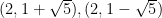
Let us illustrate these three methods and the final heuristic with a simple example. Let ![{[0,1] \times \{0\} = \{ (x,0): 0 \leq x \leq 1 \}}](https://s0.wp.com/latex.php?latex=%7B%5B0%2C1%5D+%5Ctimes+%5C%7B0%5C%7D+%3D+%5C%7B+%28x%2C0%29%3A+0+%5Cleq+x+%5Cleq+1+%5C%7D%7D&bg=ffffff&fg=000000&s=0&c=20201002)

![{[0,1]}](https://s0.wp.com/latex.php?latex=%7B%5B0%2C1%5D%7D&bg=ffffff&fg=000000&s=0&c=20201002)
Similarly, let ![{\{0\} \times [0,1] = \{ (0,y): 0 \leq y \leq 1 \}}](https://s0.wp.com/latex.php?latex=%7B%5C%7B0%5C%7D+%5Ctimes+%5B0%2C1%5D+%3D+%5C%7B+%280%2Cy%29%3A+0+%5Cleq+y+%5Cleq+1+%5C%7D%7D&bg=ffffff&fg=000000&s=0&c=20201002)

We can compute the convolution


and we thus conclude that 


In particular, ![{[0,1]^2}](https://s0.wp.com/latex.php?latex=%7B%5B0%2C1%5D%5E2%7D&bg=ffffff&fg=000000&s=0&c=20201002)
![{[0,1] \times\{0\}}](https://s0.wp.com/latex.php?latex=%7B%5B0%2C1%5D+%5Ctimes%5C%7B0%5C%7D%7D&bg=ffffff&fg=000000&s=0&c=20201002)
![{\{0\} \times [0,1]}](https://s0.wp.com/latex.php?latex=%7B%5C%7B0%5C%7D+%5Ctimes+%5B0%2C1%5D%7D&bg=ffffff&fg=000000&s=0&c=20201002)
We can arrive at the same conclusion from the regularisation method; the computations become lengthier, but more geometric in nature, and emphasises the role of transversality between the two segments supporting
![\displaystyle f_\epsilon(x,y) := \frac{1}{\epsilon} \phi(x) 1_{[0,\epsilon]}(y)](https://s0.wp.com/latex.php?latex=%5Cdisplaystyle++f_%5Cepsilon%28x%2Cy%29+%3A%3D+%5Cfrac%7B1%7D%7B%5Cepsilon%7D+%5Cphi%28x%29+1_%7B%5B0%2C%5Cepsilon%5D%7D%28y%29&bg=ffffff&fg=000000&s=0&c=20201002)
as
![\displaystyle g_\epsilon(x,y) := \frac{1}{\epsilon} 1_{[0,\epsilon]}(x) \psi(y).](https://s0.wp.com/latex.php?latex=%5Cdisplaystyle++g_%5Cepsilon%28x%2Cy%29+%3A%3D+%5Cfrac%7B1%7D%7B%5Cepsilon%7D+1_%7B%5B0%2C%5Cepsilon%5D%7D%28x%29+%5Cpsi%28y%29.&bg=ffffff&fg=000000&s=0&c=20201002)
Let us first look at the model case when ![{\phi=\psi=1_{[0,1]}}](https://s0.wp.com/latex.php?latex=%7B%5Cphi%3D%5Cpsi%3D1_%7B%5B0%2C1%5D%7D%7D&bg=ffffff&fg=000000&s=0&c=20201002)
![\displaystyle f_\epsilon = \frac{1}{\epsilon} 1_{[0,1]\times [0,\epsilon]}; \quad g_\epsilon = \frac{1}{\epsilon} 1_{[0,\epsilon] \times [0,1]}.](https://s0.wp.com/latex.php?latex=%5Cdisplaystyle++f_%5Cepsilon+%3D+%5Cfrac%7B1%7D%7B%5Cepsilon%7D+1_%7B%5B0%2C1%5D%5Ctimes+%5B0%2C%5Cepsilon%5D%7D%3B+%5Cquad+g_%5Cepsilon+%3D+%5Cfrac%7B1%7D%7B%5Cepsilon%7D+1_%7B%5B0%2C%5Cepsilon%5D+%5Ctimes+%5B0%2C1%5D%7D.&bg=ffffff&fg=000000&s=0&c=20201002)
By (1), the convolution 

where 
![\displaystyle E_\epsilon := ([0,1] \times [0,\epsilon]) \cap ((x,y) - [0,\epsilon] \times [0,1]).](https://s0.wp.com/latex.php?latex=%5Cdisplaystyle++E_%5Cepsilon+%3A%3D+%28%5B0%2C1%5D+%5Ctimes+%5B0%2C%5Cepsilon%5D%29+%5Ccap+%28%28x%2Cy%29+-+%5B0%2C%5Cepsilon%5D+%5Ctimes+%5B0%2C1%5D%29.&bg=ffffff&fg=000000&s=0&c=20201002)
When 
![{[\epsilon,1] \times [\epsilon,1]}](https://s0.wp.com/latex.php?latex=%7B%5B%5Cepsilon%2C1%5D+%5Ctimes+%5B%5Cepsilon%2C1%5D%7D&bg=ffffff&fg=000000&s=0&c=20201002)


![{[0,1+\epsilon] \times [0,1+\epsilon]}](https://s0.wp.com/latex.php?latex=%7B%5B0%2C1%2B%5Cepsilon%5D+%5Ctimes+%5B0%2C1%2B%5Cepsilon%5D%7D&bg=ffffff&fg=000000&s=0&c=20201002)
![{1_{[0,1] \times [0,1]}}](https://s0.wp.com/latex.php?latex=%7B1_%7B%5B0%2C1%5D+%5Ctimes+%5B0%2C1%5D%7D%7D&bg=ffffff&fg=000000&s=0&c=20201002)
Exercise 1 Use a similar method to verify (4) in the case that
are continuous functions on
, but one needs to invoke the Lebesgue differentiation theorem to make it run smoothly.)
Now we compute with the Fourier-analytic method. The Fourier transform 


where we abuse notation slightly by using 


so that 
and by inverting the Fourier transform we obtain (4).
Exercise 2 Let
and
be two non-parallel line segments in the plane
with vertices
. What happens in the degenerate case when
Finally, we compare the above answers with what one gets from the microlocal analysis heuristic. The measure ![{[0,1] \times \{0\}}](https://s0.wp.com/latex.php?latex=%7B%5B0%2C1%5D+%5Ctimes+%5C%7B0%5C%7D%7D&bg=ffffff&fg=000000&s=0&c=20201002)

![{x_1 \in [0,1]}](https://s0.wp.com/latex.php?latex=%7Bx_1+%5Cin+%5B0%2C1%5D%7D&bg=ffffff&fg=000000&s=0&c=20201002)


![{y_2 \in [0,1]}](https://s0.wp.com/latex.php?latex=%7By_2+%5Cin+%5B0%2C1%5D%7D&bg=ffffff&fg=000000&s=0&c=20201002)


Exercise 3 Let
in
. Use as many of the above methods as possible to establish multiple proofs of the following fact: the convolution
is an absolutely continuous multiple
of Lebesgue measure, with
supported on the ball
of radius
for
and
for
, where the implied constants are allowed to depend on the dimension
case first, which is particularly simple due to the fact that the addition map
is mostly a local diffeomorphism. The Fourier-based approach is instructive, but requires either asymptotics of Bessel functions or the principle of stationary phase.)

[Note: the content of this post is standard number theoretic material that can be found in many textbooks (I am relying principally here on Iwaniec and Kowalski); I am not claiming any new progress on any version of the Riemann hypothesis here, but am simply arranging existing facts together.]
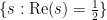
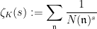
The Riemann hypothesis is arguably the most important and famous unsolved problem in number theory. It is usually phrased in terms of the Riemann zeta function 

for 

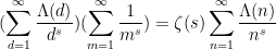
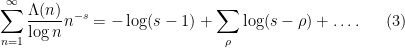
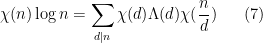
One of the main reasons that the Riemann hypothesis is so important to number theory is that the zeroes of the zeta function in the critical strip control the distribution of the primes. To see the connection, let us perform the following formal manipulations (ignoring for now the important analytic issues of convergence of series, interchanging sums, branches of the logarithm, etc., in order to focus on the intuition). The starting point is the fundamental theorem of arithmetic, which asserts that every natural number 

for any natural number 


formally at least. Writing 
whereas the left-hand side is (formally, at least) equal to 
(formally, at least). If we integrate this, we are formally led to the identity
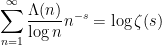
or equivalently to the exponential identity

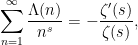
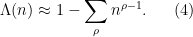
which allows one to reconstruct the Riemann zeta function from the von Mangoldt function. (It is instructive exercise in enumerative combinatorics to try to prove this identity directly, at the level of formal Dirichlet series, using the fundamental theorem of arithmetic of course.) Now, as 


(where we will be intentionally vague about what is hiding in the 
Note that
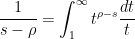
and hence on integrating in
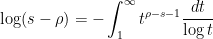
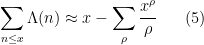
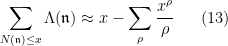
and thus we have the heuristic approximation
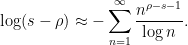
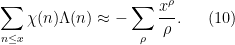
Comparing this with (3), we are led to a heuristic form of the explicit formula
When trying to make this heuristic rigorous, it turns out (due to the rough nature of both sides of (4)) that one has to interpret the explicit formula in some suitably weak sense, for instance by testing (4) against the indicator function ![{1_{[0,x]}(n)}](https://s0.wp.com/latex.php?latex=%7B1_%7B%5B0%2Cx%5D%7D%28n%29%7D&bg=ffffff&fg=000000&s=0&c=20201002)
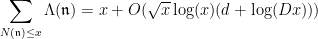
which can in fact be made into a rigorous statement after some truncation (the von Mangoldt explicit formula). From this formula we now see how helpful the Riemann hypothesis will be to control the distribution of the primes; indeed, if the Riemann hypothesis holds, so that 

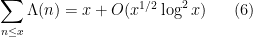
as 

for any fixed 

can be automatically amplified to the stronger bound

with both bounds being equivalent to the Riemann hypothesis. Of course, the Riemann hypothesis for the Riemann zeta function remains open; but partial progress on this hypothesis (in the form of zero-free regions for the zeta function) leads to partial versions of the asymptotic (6). For instance, it is known that there are no zeroes of the zeta function on the line 

see e.g. this previous blog post for more discussion.
The main engine powering the above observations was the fundamental theorem of arithmetic, and so one can expect to establish similar assertions in other contexts where some version of the fundamental theorem of arithmetic is available. One of the simplest such variants is to continue working on the natural numbers, but “twist” them by a Dirichlet character 

and essentially the same manipulations as before eventually lead to the exponential identity

which is a twisted version of (2), as well as twisted explicit formula, which heuristically takes the form
for non-principal 

(See e.g. Davenport’s book for a more rigorous discussion which emphasises the analogy between the Riemann zeta function and the Dirichlet 

for any non-principal Dirichlet character

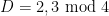
(where 


![{K = {\bf Q}[\sqrt{D}]}](https://s0.wp.com/latex.php?latex=%7BK+%3D+%7B%5Cbf+Q%7D%5B%5Csqrt%7BD%7D%5D%7D&bg=ffffff&fg=000000&s=0&c=20201002)

![{{\mathcal O}_K = {\bf Z}[\omega]}](https://s0.wp.com/latex.php?latex=%7B%7B%5Cmathcal+O%7D_K+%3D+%7B%5Cbf+Z%7D%5B%5Comega%5D%7D&bg=ffffff&fg=000000&s=0&c=20201002)


![{{\bf Z}[\omega]}](https://s0.wp.com/latex.php?latex=%7B%7B%5Cbf+Z%7D%5B%5Comega%5D%7D&bg=ffffff&fg=000000&s=0&c=20201002)


![{{\bf Z}[\sqrt{-5}]}](https://s0.wp.com/latex.php?latex=%7B%7B%5Cbf+Z%7D%5B%5Csqrt%7B-5%7D%5D%7D&bg=ffffff&fg=000000&s=0&c=20201002)


where the summation is over all non-trivial ideals in 


which leads as before to an exponential identity

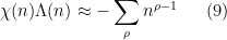
and an explicit formula of the heuristic form

in analogy with (5) or (10). Again, a suitable Riemann hypothesis for the Dedekind zeta function leads to good asymptotics for the distribution of prime ideals, giving a bound of the form
where 

where
As was the case with the Dirichlet
Very analogous considerations hold if we move from number fields to function fields. The simplest case is the function field associated to the affine line 


![{{\mathbb F}[t]}](https://s0.wp.com/latex.php?latex=%7B%7B%5Cmathbb+F%7D%5Bt%5D%7D&bg=ffffff&fg=000000&s=0&c=20201002)

![{{\mathbb F}[t] / (f)}](https://s0.wp.com/latex.php?latex=%7B%7B%5Cmathbb+F%7D%5Bt%5D+%2F+%28f%29%7D&bg=ffffff&fg=000000&s=0&c=20201002)
Because of this, we will normalise things slightly differently here and use 


where 


and 

We have the analogue of (1) (or (7) or (11)):
which leads as before to an exponential identity

analogous to (2), (8), or (12). It also leads to the explicit formula
where 

where 

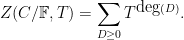
As it turns out, in the function field setting, the zeta functions are always rational (this is part of the Weil conjectures), and the above heuristic formula is basically exact up to a constant factor, thus
for an explicit integer 


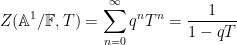
so in fact there are no zeroes whatsoever, and no pole at
Among other things, this tells us that the number of irreducible monic polynomials of degree 
We can transition from an algebraic perspective to a geometric one, by viewing a given monic polynomial ![{f \in {\mathbb F}[t]}](https://s0.wp.com/latex.php?latex=%7Bf+%5Cin+%7B%5Cmathbb+F%7D%5Bt%5D%7D&bg=ffffff&fg=000000&s=0&c=20201002)


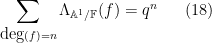
Now consider the degree 


The identity (18) thus is equivalent to the thoroughly boring fact that the number of 

for some suitable 
![{{\mathbb F}[x,y] / (y^2-x^3-ax-b)}](https://s0.wp.com/latex.php?latex=%7B%7B%5Cmathbb+F%7D%5Bx%2Cy%5D+%2F+%28y%5E2-x%5E3-ax-b%29%7D&bg=ffffff&fg=000000&s=0&c=20201002)

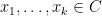
and a von Mangoldt function 


![{[x_1] + \ldots + [x_k]}](https://s0.wp.com/latex.php?latex=%7B%5Bx_1%5D+%2B+%5Cldots+%2B+%5Bx_k%5D%7D&bg=ffffff&fg=000000&s=0&c=20201002)
where the sum is over effective rational divisors
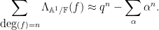
The analogue of (19), which gives a geometric interpretation to sums of the von Mangoldt function, becomes


thus this sum is simply counting the number of

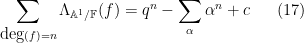
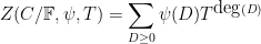
and the analogue of the explicit formula (17) (or (5), (10) or (13)) is
where 

To evaluate 

for two complex numbers
The Riemann hypothesis for (untwisted) curves – which is the deepest and most difficult aspect of the Weil conjectures for these curves – asserts that the zeroes of 


where the implied constant depends only on the genus of
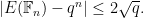
As before, we have an important amplification phenomenon: if we can establish a weaker estimate, e.g.

then we can automatically deduce the stronger bound (23). This amplification is not a mere curiosity; most of the proofs of the Riemann hypothesis for curves proceed via this fact. For instance, by using the elementary method of Stepanov to bound points in curves (discussed for instance in this previous post), one can establish the preliminary bound (24) for large 
Much as the Riemann zeta function can be twisted by a Dirichlet character to form a Dirichlet 


![{D = [x_1] + \ldots + [x_k]}](https://s0.wp.com/latex.php?latex=%7BD+%3D+%5Bx_1%5D+%2B+%5Cldots+%2B+%5Bx_k%5D%7D&bg=ffffff&fg=000000&s=0&c=20201002)


![\displaystyle \psi( [x_1] + \ldots + [x_k] ) := \psi( x_1 + \ldots + x_k )](https://s0.wp.com/latex.php?latex=%5Cdisplaystyle++%5Cpsi%28+%5Bx_1%5D+%2B+%5Cldots+%2B+%5Bx_k%5D+%29+%3A%3D+%5Cpsi%28+x_1+%2B+%5Cldots+%2B+x_k+%29&bg=ffffff&fg=000000&s=0&c=20201002)
and observe that 


then by twisting the previous analysis, we eventually arrive at the exponential identity

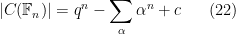
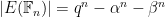
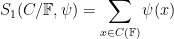
in analogy with (21) (or (2), (8), (12), or (16)), where the companion sums 
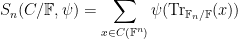
where the trace 


In particular, 
which is an important type of sum in analytic number theory, containing for instance the Kloosterman sum
as a special case, where 


If 


for the companion sums, where 

for all 


for the companion sums (and in particular gives the very explicit Weil bound 

As before, most of the known proofs of the Riemann hypothesis for these twisted zeta functions proceed by first establishing this weaker bound (e.g. one could again use Stepanov’s method here for this goal) and then amplifying to the full bound (28); see Chapter 11 of Iwaniec-Kowalski for further details.
One can also twist the zeta function on a curve by a multiplicative character 
![{[x_1]+\ldots+[x_k]}](https://s0.wp.com/latex.php?latex=%7B%5Bx_1%5D%2B%5Cldots%2B%5Bx_k%5D%7D&bg=ffffff&fg=000000&s=0&c=20201002)


by the norm

Again, see Chapter 11 of Iwaniec-Kowalski for details.
Deligne famously extended the above theory to higher-dimensional varieties than curves, and also to the closely related context of 
Let 


One can remove the logarithm by using some number theoretic constructions. For instance, if 


As it turns out, this construction is close to optimal, in that there is a polynomial limit to how many unit vectors one can pack into
Theorem 1 (Cheap Kabatjanskii-Levenstein bound) Let
for some
. Then we have
for some absolute constant
In particular, for fixed 


Note that for 


As I learned recently from Philippe Michel, a more precise version of this theorem is due to Kabatjanskii and Levenstein, who studied the closely related problem of sphere packing (or more precisely, cap packing) in the unit sphere
We begin with an easy case, basically the
Lemma 2 Let
for all distinct
.
Proof: Suppose for contradiction that 


But by hypothesis, the left-hand side is at most 
To amplify the above lemma to cover larger values of
Corollary 3 Let
for all distinct
.
Proof: We work in the symmetric component 


Using the trivial bound 

We can thus prove Theorem 1 by setting 
Van Vu and I have just uploaded to the arXiv our joint paper “Local universality of zeroes of random polynomials“. This paper is a sequel to our previous work on local universality of eigenvalues of (non-Hermitian) random matrices 


where 


Our results are fairly general with regard to the choice of coefficients 
- Flat polynomials (or Weyl polynomials) in which
.
- Elliptic polynomials (or binomial polynomials) in which
.
- Kac polynomials in which
.
The flat and elliptic polynomials enjoy special symmetries in the model case when the atom distribution 


The global (i.e. coarse-scale) distribution of zeroes of these polynomials is well understood, first in the case of gaussian distributions using the fundamental tool of the Kac-Rice formula, and then for more general choices of atom distribution in the recent work of Kabluchko and Zaporozhets. The zeroes of the flat polynomials are asymptotically distributed according to the circular law, normalised to be uniformly distributed on the disk 


Similarly, the distribution of the elliptic polynomials is known to be asymptotically distributed according to a Cauchy-type distribution 


In our paper we studied the local distribution of zeroes at the scale of the typical spacing. In the case of polynomials with continuous complex atom disribution 


We also have analogous results in the case of polynomials with real coefficients (so that the coefficients 


While our methods are based on our earlier work on eigenvalues of random matrices, the situation with random polynomials is actually somewhat easier to deal with. This is because the log-magnitude 
The purpose of this post is to link to a short unpublished note of mine that I wrote back in 2010 but forgot to put on my web page at the time. Entitled “A physical space proof of the bilinear Strichartz and local smoothing estimates for the Schrodinger equation“, it gives a proof of two standard estimates for the free (linear) Schrodinger equation in flat Euclidean space, namely the bilinear Strichartz estimate and the local smoothing estimate, using primarily “physical space” methods such as integration by parts, instead of “frequency space” methods based on the Fourier transform, although a small amount of Fourier analysis (basically sectoral projection to make the Schrodinger waves move roughly in a given direction) is still needed. This is somewhat in the spirit of an older paper of mine with Klainerman and Rodnianski doing something similar for the wave equation, and is also very similar to a paper of Planchon and Vega from 2009. The hope was that by avoiding the finer properties of the Fourier transform, one could obtain a more robust argument which could also extend to nonlinear, non-free, or non-flat situations. These notes were cited once or twice by some people that I had privately circulated them to, so I decided to put them online here for reference.
UPDATE, July 24: Fabrice Planchon has kindly supplied another note in which he gives a particularly simple proof of local smoothing in one dimension, and discusses some other variants of the method (related to the paper of Planchon and Vega cited earlier).
As in previous posts, we use the following asymptotic notation:
The purpose of this post is to collect together all the various refinements to the second half of Zhang’s paper that have been obtained as part of the polymath8 project and present them as a coherent argument. In order to state the main result, we need to recall some definitions. If 


for all coprime 


If 
![{[y^{-1} R, R]}](https://s0.wp.com/latex.php?latex=%7B%5By%5E%7B-1%7D+R%2C+R%5D%7D&bg=ffffff&fg=000000&s=0&c=20201002)

Given any finitely supported sequence
For any fixed ![{MPZ''[\varpi,\delta]}](https://s0.wp.com/latex.php?latex=%7BMPZ%27%27%5B%5Cvarpi%2C%5Cdelta%5D%7D&bg=ffffff&fg=000000&s=0&c=20201002)
![\displaystyle \sum_{q \in {\mathcal S}_I \cap {\mathcal D}_{x^\delta}^2: q \leq x^{1/2+2\varpi}} |\Delta(\Lambda 1_{[x,2x]}; a\ (q))| \ll x \log^{-A} x \ \ \ \ \ (1)](https://s0.wp.com/latex.php?latex=%5Cdisplaystyle++%5Csum_%7Bq+%5Cin+%7B%5Cmathcal+S%7D_I+%5Ccap+%7B%5Cmathcal+D%7D_%7Bx%5E%5Cdelta%7D%5E2%3A+q+%5Cleq+x%5E%7B1%2F2%2B2%5Cvarpi%7D%7D+%7C%5CDelta%28%5CLambda+1_%7B%5Bx%2C2x%5D%7D%3B+a%5C+%28q%29%29%7C+%5Cll+x+%5Clog%5E%7B-A%7D+x+%5C+%5C+%5C+%5C+%5C+%281%29&bg=ffffff&fg=000000&s=0&c=20201002)
for any fixed
This improves upon the previous constraint of 


This estimate is deduced from three sub-estimates, which require a bit more notation to state. We need a fixed quantity 
Definition 2 A coefficient sequence is a finitely supported sequence
for all
- (i) A coefficient sequence
.
- (ii) A coefficient sequence
for any
- (iii) A coefficient sequence
) is said to be smooth if it takes the form
obeying the derivative bounds
for all fixed


Definition 3 (Type I, Type II, Type III estimates) Let
- (i) We say that
holds if, whenever
and
for some fixed
- (ii) We say that
holds if the conclusion (7) of
for some sufficiently small fixed
- (iii) We say that
holds if, whenever
are quantities with
and
are coefficient sequences at scales
respectively, with
smooth, we have


Theorem 1 is then a consequence of the following four statements.
Theorem 4 (Type I estimate)
are fixed quantities such that

Theorem 5 (Type II estimate)
are fixed quantities such that

Theorem 6 (Type III estimate)
are fixed quantities such that
In particular, if
then all values of

Lemma 7 (Combinatorial lemma) Let
be such that
Indeed, if 
The proofs of Theorems 4, 5, 6 will be given below the fold, while the proof of Lemma 7 follows from the arguments in this previous post. We remark that in our current arguments, the double dense divisibility is only fully used in the Type I estimates; the Type II and Type III estimates are also valid just with single dense divisibility.
Remark 1 Theorem 6 is vacuously true for
, as the condition (10) cannot be satisfied in this case. If we use this trivial case of Theorem 6, while keeping the full strength of Theorems 4 and 5, we obtain Theorem 1 in the regime

Recent Comments