
You are currently browsing the tag archive for the ‘ergodic theory’ tag.
Asgar Jamneshan and I have just uploaded to the arXiv our paper “An uncountable Moore-Schmidt theorem“. This paper revisits a classical theorem of Moore and Schmidt in measurable cohomology of measure-preserving systems. To state the theorem, let 


Let 


Let 


for 


This connection with group extensions was the original motivation for our study of measurable cohomology, but is not the focus of the current paper.
A special case of a 


for 


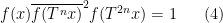
Theorem 1 (Countable Moore-Schmidt theorem) Let
- (i)
- (ii)
- (iii)
Then a
, the
-valued cocycles
are concrete coboundaries.
The hypotheses (i), (ii), (iii) are saying in some sense that the data 
Let us very briefly sketch the main ideas of the proof of Theorem 1. Ignore for now issues of measurability, and pretend that something that holds almost everywhere in fact holds everywhere. The hard direction is to show that if each 


for all 

for all 
Comparing the two equations, the task would be easy if we could find an

for all 


for all 

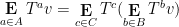
Now, it turns out that one cannot derive the equation (4) directly from the given information (2). However, the left-hand side of (2) is additive in

In other words, we don’t get to show that the left-hand side of (4) vanishes, but we do at least get to show that it is

for some constants 
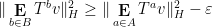
Now we need to eliminate the constants. This can be done by the following group-theoretic projection. Let 


then from (5) we see that

while from (2) one has

and now the previous strategy works with 

In making the above argument rigorous, the hypotheses (i)-(iii) are used in several places. For instance, to reduce to the ergodic case one relies on the ergodic decomposition, which requires the hypothesis (ii). Also, most of the above equations only hold outside of a set of measure zero, and the hypothesis (i) and the hypothesis (iii) (which is equivalent to
My co-author Asgar Jamneshan and I are working on a long-term project to extend many results in ergodic theory (such as the aforementioned Host-Kra structure theorem) to “uncountable” settings in which hypotheses analogous to (i)-(iii) are omitted; thus we wish to consider actions on uncountable groups, on spaces that are not standard Borel, and cocycles taking values in groups that are not metrisable. Such uncountable contexts naturally arise when trying to apply ergodic theory techniques to combinatorial problems (such as the inverse conjecture for the Gowers norms), as one often relies on the ultraproduct construction (or something similar) to generate an ergodic theory translation of these problems, and these constructions usually give “uncountable” objects rather than “countable” ones. (For instance, the ultraproduct of finite groups is a hyperfinite group, which is usually uncountable.). This paper marks the first step in this project by extending the Moore-Schmidt theorem to the uncountable setting.
If one simply drops the hypotheses (i)-(iii) and tries to prove the Moore-Schmidt theorem, several serious difficulties arise. We have already mentioned the loss of the ergodic decomposition and the possibility that one has to control an uncountable union of null sets. But there is in fact a more basic problem when one deletes (iii): the addition operation 


would be measurable in 


To resolve this problem, we give 


Passing to the Baire 


Every concrete measurable space 


![{[f]: X_\mu \rightarrow Y}](https://s0.wp.com/latex.php?latex=%7B%5Bf%5D%3A+X_%5Cmu+%5Crightarrow+Y%7D&bg=ffffff&fg=000000&s=0&c=20201002)
Theorem 2 (Uncountable Moore-Schmidt theorem) Let
With the abstract formalism, the proof of the uncountable Moore-Schmidt theorem is almost identical to the countable one (in fact we were able to make some simplifications, such as avoiding the use of the ergodic decomposition). A key tool is what we call a “conditional Pontryagin duality” theorem, which asserts that if one has an abstract measurable map 


We feel that it is natural to stay within the abstract measure theory formalism whenever dealing with uncountable situations. However, it is still an interesting question as to when one can guarantee that the abstract objects constructed in this formalism are representable by concrete analogues. The basic questions in this regard are:
- (i) Suppose one has an abstract measurable map
into a concrete measurable space. Does there exist a representation of
by a concrete measurable map
? Is it unique up to almost everywhere equivalence?
- (ii) Suppose one has a concrete cocycle that is an abstract coboundary. When can it be represented by a concrete coboundary?
For (i) the answer is somewhat interesting (as I learned after posing this MathOverflow question):
- If
does not separate points, or is not compact metrisable or Polish, there can be counterexamples to uniqueness. If
- If
- If
- If
- If
- For more general
to
(or, in the language of abstract measurable spaces, the existence of an abstract retraction from
- It is a long-standing open question (posed for instance by Fremlin) whether it is relatively consistent with ZFC that existence holds whenever
Our understanding of (ii) is much less complete:
- If
- If
In view of the answers to (i), I would not be surprised if the full answer to (ii) was also sensitive to axioms of set theory. However, such set theoretic issues seem to be almost completely avoided if one sticks with the abstract formalism throughout; they only arise when trying to pass back and forth between the abstract and concrete categories.
Let 


A measure-preserving system is said to be ergodic if all the invariant sets are either zero measure or full measure. An equivalent form of this statement is that any measurable function 


In this short note I would like to use the mean ergodic theorem to show that ergodic systems also have the property that “somewhat locally constant” functions are necessarily “somewhat globally constant”; this is not a deep observation, and probably already in the literature, but I found it a cute statement that I had not previously seen. More precisely:
Corollary 1 Let
for some
. Then there exists a constant
for
.

Informally: if 
Proof: By composing 


For each 
Using the ergodic theorem, we conclude that

On the other hand, 


By the Bolzano-Weierstrass theorem, we may pass to a subsequence where 

for infinitely many

The claim follows.

The von Neumann ergodic theorem (the Hilbert space version of the mean ergodic theorem) asserts that if 


in the strong topology, where 


for any Folner sequence 


In a previous blog post, I noted a variant of this ergodic theorem (due to Alaoglu and Birkhoff) that holds even when the group
Theorem 1 (Abstract ergodic theorem) Let
in this closed convex hull.
I recently stumbled upon a different way to think about this theorem, in the additive case 


Note that the multiplicity function of the set 
We can define a directed set on 


When
We can then give an alternate formulation of the abstract ergodic theorem in the abelian case:
Theorem 2 (Abelian abstract ergodic theorem) Let
in the strong topology of
Proof: Suppose that 
so by unitarity and the triangle inequality we have

thus 


for all 
We can write

and so from the parallelogram law and unitarity we have
for all 

for any 

and hence 


and thus on taking strong limits

and so 
To relate this result to the classical ergodic theorem, we observe
Lemma 3 Let
, and let
be a bounded sequence in a normed vector space indexed by
exists, then
exists, and the two limits are equal.
Proof: From the F{\o}lner property, we see that for any 


It turns out that this approach can also be used as an alternate way to construct the Gowers–Host-Kra seminorms in ergodic theory, which has the feature that it does not explicitly require any amenability on the group
Given an arbitrary additive group 


in the strong topology of 


In a similar spirit, we have
Theorem 4 (Convergence of Gowers-Host-Kra seminorms) Let
be a
be a natural number, and for every
, let
, which for simplicity we take to be real-valued. Then the expression
converges, where we write
, and we are using the product direct set on
to define the convergence
. In particular, for
, the limit
converges.

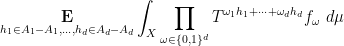

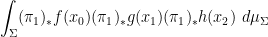
We prove this theorem below the fold. It implies a number of other known descriptions of the Gowers-Host-Kra seminorms 

for 

This definition also manifestly demonstrates the cube symmetries of the Host-Kra measures ![{\mu^{[d]}}](https://s0.wp.com/latex.php?latex=%7B%5Cmu%5E%7B%5Bd%5D%7D%7D&bg=ffffff&fg=000000&s=0&c=20201002)

![\displaystyle \langle (f_\omega)_{\omega \in \{0,1\}^d} \rangle_{U^d({\mathrm X})} = \int_{X^{\{0,1\}^d}} \bigotimes_{\omega \in \{0,1\}^d} f_\omega\ d\mu^{[d]}.](https://s0.wp.com/latex.php?latex=%5Cdisplaystyle+%5Clangle+%28f_%5Comega%29_%7B%5Comega+%5Cin+%5C%7B0%2C1%5C%7D%5Ed%7D+%5Crangle_%7BU%5Ed%28%7B%5Cmathrm+X%7D%29%7D+%3D+%5Cint_%7BX%5E%7B%5C%7B0%2C1%5C%7D%5Ed%7D%7D+%5Cbigotimes_%7B%5Comega+%5Cin+%5C%7B0%2C1%5C%7D%5Ed%7D+f_%5Comega%5C+d%5Cmu%5E%7B%5Bd%5D%7D.&bg=ffffff&fg=000000&s=0&c=20201002)
In a subsequent blog post I hope to present a more detailed study of the 

As laid out in the foundational work of Kolmogorov, a classical probability space (or probability space for short) is a triplet 
![{\mu: {\mathcal X} \rightarrow [0,1]}](https://s0.wp.com/latex.php?latex=%7B%5Cmu%3A+%7B%5Cmathcal+X%7D+%5Crightarrow+%5B0%2C1%5D%7D&bg=ffffff&fg=000000&s=0&c=20201002)
- the (real) Hilbert space
of square-integrable functions
; and
- the unital commutative Banach algebra
of essentially bounded functions
defined as the essential supremum of
.
There is also a trace 

One can form the category 


Let us now abstract the algebraic features of these spaces as follows; for want of a better name, I will refer to this abstraction as an algebraic probability space, and is very similar to the non-commutative probability spaces studied in this previous post, except that these spaces are now commutative (and real).
Definition 1 An algebraic probability space is a pair
where
is a unital commutative real algebra;
is a homomorphism such that
and
for all
;
- Every element
. (Technically, this isn’t an algebraic property, but I need it for technical reasons.)
A morphism
is a homomorphism
which is trace-preserving, in the sense that
for all
.
For want of a better name, I’ll denote the category of algebraic probability spaces as 


By the previous discussion, we have a covariant functor 

for 
In this post I would like to describe a functor 
Let us describe how to construct the functor
- Starting with an algebraic probability space
, and also form the spectral radius
.
- The inner product is clearly positive semi-definite. Quotienting out the null vectors and taking completions, we arrive at a real Hilbert space
, to which the trace
may be extended.
- Somewhat less obviously, the spectral radius is well-defined and gives a norm on
of
- The idempotents
of the Banach algebra
.
- The Boolean algebra homomorphisms
(or equivalently, the real algebra homomorphisms
) may be indexed by elements
- Let
for every
.
- Let
be the
, where
is a sequence with
.
- One verifies that
. Using this isomorphism, the trace
, and the abstract spaces
may now be identified with their concrete counterparts
- Every algebraic probability space morphism
generates a classical probability morphism
via the formula
using a pullback operation
on the abstract
that can be defined by density.
Remark 1 The classical probability space
The partial inversion relationship between the functors
- There is a natural transformation from
to the identity functor
.
More informally: if one starts with an algebraic probability space 


Remark 2 The opposite composition
is a little odd: it takes an arbitrary probability space
, with
being the space of homomorphisms
. while there is “morally” an embedding of
,
, then these algebras become naturally isomorphic after quotienting out by null sets.
Remark 3 An algebraic probability space captures a bit more structure than a classical probability space, because
(with the usual Haar measure and the usual trace
), any unital subalgebra
that is dense in
will generate the same classical probability space
of homomorphisms from
(with the measure induced from
, the Wiener algebra
or the full space
of continuous functions on a topological space. I hope to discuss one such example of extra structure (coming from the Gowers-Host-Kra theory of uniformity seminorms) in a later blog post (this generalises the example of the Wiener algebra given previously, which is encoding “Fourier structure”).
A small example of how one could use the functors 


More indirectly, the functors
There are a number of ways to construct the real numbers
- as the metric completion of
(thus,
- as the space of Dedekind cuts on the rationals
- as the space of quasimorphisms
on the integers, quotiented by bounded functions. (I believe this construction first appears in this paper of Street, who credits the idea to Schanuel, though the germ of this construction arguably goes all the way back to Eudoxus.)
There is also a fourth family of constructions that proceeds via nonstandard analysis, as a special case of what is known as the nonstandard hull construction. (Here I will assume some basic familiarity with nonstandard analysis and ultraproducts, as covered for instance in this previous blog post.) Given an unbounded nonstandard natural number 

- The group
of all nonstandard integers of magnitude less than or comparable to
; and
- The group
of nonstandard integers of magnitude infinitesimally smaller than
The group 


Proposition 1 For any coset
of
with the property that
. The map
is then an isomorphism between the additive groups
Proof: Uniqueness is clear. For existence, observe that the set 
In a similar vein, we can view the unit interval ![{[0,1]}](https://s0.wp.com/latex.php?latex=%7B%5B0%2C1%5D%7D&bg=ffffff&fg=000000&s=0&c=20201002)
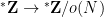
![\displaystyle [0,1] \equiv [N] / o(N) \ \ \ \ \ (1)](https://s0.wp.com/latex.php?latex=%5Cdisplaystyle++%5B0%2C1%5D+%5Cequiv+%5BN%5D+%2F+o%28N%29+%5C+%5C+%5C+%5C+%5C+%281%29&bg=ffffff&fg=000000&s=0&c=20201002)
where ![{[N]}](https://s0.wp.com/latex.php?latex=%7B%5BN%5D%7D&bg=ffffff&fg=000000&s=0&c=20201002)
![{[N]/o(N)}](https://s0.wp.com/latex.php?latex=%7B%5BN%5D%2Fo%28N%29%7D&bg=ffffff&fg=000000&s=0&c=20201002)


In this post I would like to record a nice measure-theoretic version of the equivalence (1), which essentially appears already in standard texts on Loeb measure (see e.g. this text of Cutland). To describe the results, we must first quickly recall the construction of Loeb measure on 

This is a finitely additive probability measure on the Boolean algebra of internal subsets of 
![{A \subset [N]}](https://s0.wp.com/latex.php?latex=%7BA+%5Csubset+%5BN%5D%7D&bg=ffffff&fg=000000&s=0&c=20201002)
where 


![{([N], {\mathcal L}, \mu)}](https://s0.wp.com/latex.php?latex=%7B%28%5BN%5D%2C+%7B%5Cmathcal+L%7D%2C+%5Cmu%29%7D&bg=ffffff&fg=000000&s=0&c=20201002)
Now, the group 
![{n \in [N]}](https://s0.wp.com/latex.php?latex=%7Bn+%5Cin+%5BN%5D%7D&bg=ffffff&fg=000000&s=0&c=20201002)


![{Z^0_{o(N)}([N]) = ([N], {\mathcal L}^{o(N)}, \mu\downharpoonright_{{\mathcal L}^{o(N)}})}](https://s0.wp.com/latex.php?latex=%7BZ%5E0_%7Bo%28N%29%7D%28%5BN%5D%29+%3D+%28%5BN%5D%2C+%7B%5Cmathcal+L%7D%5E%7Bo%28N%29%7D%2C+%5Cmu%5Cdownharpoonright_%7B%7B%5Cmathcal+L%7D%5E%7Bo%28N%29%7D%7D%29%7D&bg=ffffff&fg=000000&s=0&c=20201002)

The claim is then that this invariant factor is equivalent (up to almost everywhere equivalence) to the unit interval 
Theorem 2 Given a set
, there exists a Lebesgue measurable set
, unique up to
. Conversely, if
is Lebesgue measurable, then
is in
, and
.
More informally, we have the measure-theoretic version
![\displaystyle [0,1] \equiv Z^0_{o(N)}( [N] )](https://s0.wp.com/latex.php?latex=%5Cdisplaystyle++%5B0%2C1%5D+%5Cequiv+Z%5E0_%7Bo%28N%29%7D%28+%5BN%5D+%29&bg=ffffff&fg=000000&s=0&c=20201002)
of (1).
Proof: We first prove the converse. It is clear that 

![{E \subset [0,1]}](https://s0.wp.com/latex.php?latex=%7BE+%5Csubset+%5B0%2C1%5D%7D&bg=ffffff&fg=000000&s=0&c=20201002)
Now we establish the forward claim. Uniqueness is clear from the converse claim, so it suffices to show existence. Let ![{A_\epsilon \subset [N]}](https://s0.wp.com/latex.php?latex=%7BA_%5Cepsilon+%5Csubset+%5BN%5D%7D&bg=ffffff&fg=000000&s=0&c=20201002)


![{f_\epsilon: [N] \rightarrow {}^* {\bf R}}](https://s0.wp.com/latex.php?latex=%7Bf_%5Cepsilon%3A+%5BN%5D+%5Crightarrow+%7B%7D%5E%2A+%7B%5Cbf+R%7D%7D&bg=ffffff&fg=000000&s=0&c=20201002)
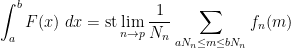
![\displaystyle f(n) := \hbox{st} \frac{1}{\delta N} \sum_{m \in [N]: m \leq n \leq m+\delta N} 1_{A_\epsilon}(m),](https://s0.wp.com/latex.php?latex=%5Cdisplaystyle++f%28n%29+%3A%3D+%5Chbox%7Bst%7D+%5Cfrac%7B1%7D%7B%5Cdelta+N%7D+%5Csum_%7Bm+%5Cin+%5BN%5D%3A+m+%5Cleq+n+%5Cleq+m%2B%5Cdelta+N%7D+1_%7BA_%5Cepsilon%7D%28m%29%2C&bg=ffffff&fg=000000&s=0&c=20201002)
then from the (nonstandard) triangle inequality we have
![\displaystyle \frac{1}{N} \sum_{n \in [N]} |f(n) - 1_{A_\epsilon}(n)| \leq 3\epsilon](https://s0.wp.com/latex.php?latex=%5Cdisplaystyle++%5Cfrac%7B1%7D%7BN%7D+%5Csum_%7Bn+%5Cin+%5BN%5D%7D+%7Cf%28n%29+-+1_%7BA_%5Cepsilon%7D%28n%29%7C+%5Cleq+3%5Cepsilon&bg=ffffff&fg=000000&s=0&c=20201002)
(say). On the other hand,
and so in particular we see that
for some Lipschitz continuous function ![{\tilde f: [0,1] \rightarrow [0,1]}](https://s0.wp.com/latex.php?latex=%7B%5Ctilde+f%3A+%5B0%2C1%5D+%5Crightarrow+%5B0%2C1%5D%7D&bg=ffffff&fg=000000&s=0&c=20201002)


Thanks to the Lebesgue differentiation theorem, the conditional expectation ![{{\bf E}( f | Z^0_{o(N)}([N]))}](https://s0.wp.com/latex.php?latex=%7B%7B%5Cbf+E%7D%28+f+%7C+Z%5E0_%7Bo%28N%29%7D%28%5BN%5D%29%29%7D&bg=ffffff&fg=000000&s=0&c=20201002)
![{f: [N] \rightarrow {\bf R}}](https://s0.wp.com/latex.php?latex=%7Bf%3A+%5BN%5D+%5Crightarrow+%7B%5Cbf+R%7D%7D&bg=ffffff&fg=000000&s=0&c=20201002)
![\displaystyle {\bf E}( f | Z^0_{o(N)}([N]))(x) := \lim_{\epsilon \rightarrow 0} \frac{1}{2\epsilon} \int_{[x-\epsilon N,x+\epsilon N]} f\ d\mu.](https://s0.wp.com/latex.php?latex=%5Cdisplaystyle++%7B%5Cbf+E%7D%28+f+%7C+Z%5E0_%7Bo%28N%29%7D%28%5BN%5D%29%29%28x%29+%3A%3D+%5Clim_%7B%5Cepsilon+%5Crightarrow+0%7D+%5Cfrac%7B1%7D%7B2%5Cepsilon%7D+%5Cint_%7B%5Bx-%5Cepsilon+N%2Cx%2B%5Cepsilon+N%5D%7D+f%5C+d%5Cmu.&bg=ffffff&fg=000000&s=0&c=20201002)
By the abstract ergodic theorem from the previous post, one can also view this conditional expectation as the element in the closed convex hull of the shifts 


If ![{f: [N] \rightarrow [-1,1]}](https://s0.wp.com/latex.php?latex=%7Bf%3A+%5BN%5D+%5Crightarrow+%5B-1%2C1%5D%7D&bg=ffffff&fg=000000&s=0&c=20201002)
![{f_n: [N_n] \rightarrow [-1,1]}](https://s0.wp.com/latex.php?latex=%7Bf_n%3A+%5BN_n%5D+%5Crightarrow+%5B-1%2C1%5D%7D&bg=ffffff&fg=000000&s=0&c=20201002)
![{F := {\bf E}( f | Z^0_{o(N)}([N]))}](https://s0.wp.com/latex.php?latex=%7BF+%3A%3D+%7B%5Cbf+E%7D%28+f+%7C+Z%5E0_%7Bo%28N%29%7D%28%5BN%5D%29%29%7D&bg=ffffff&fg=000000&s=0&c=20201002)

![{F: [0,1] \rightarrow [-1,1]}](https://s0.wp.com/latex.php?latex=%7BF%3A+%5B0%2C1%5D+%5Crightarrow+%5B-1%2C1%5D%7D&bg=ffffff&fg=000000&s=0&c=20201002)
for all 


thus ![{[N_n]}](https://s0.wp.com/latex.php?latex=%7B%5BN_n%5D%7D&bg=ffffff&fg=000000&s=0&c=20201002)

I’m continuing to look into understanding the ergodic theory of
Vitaly Bergelson, Tamar Ziegler, and I have just uploaded to the arXiv our joint paper “Multiple recurrence and convergence results associated to 


converges as 

see e.g. this previous blog post. Informally, one can interpret this limit formula as an equidistribution result: if 


If we allow 


where 


Limit formulae are known for multiple ergodic averages as well, although the statement becomes more complicated. For instance, consider the expression

for three functions 


which would roughly speaking correspond to an assertion that the triplet 


tying together 


where 

and 


If one considers a quadruple average
(analogous to counting length four progressions) then the situation becomes more complicated still, even in the ergodic case. In addition to the (linear) eigenfunctions that already showed up in the computation of the triple average (3), a new type of constraint also arises from quadratic eigenfunctions 

between 
The above discussion was concerned with 


As a consequence, we can recover finite field analogues of most of the results of Bergelson-Host-Kra, though interestingly some of the counterexamples demonstrating sharpness of their results for

for a syndetic set of 


One of the basic objects of study in combinatorics are finite strings 


On the other hand, the basic object of study in dynamics (and in related fields, such as ergodic theory) is that of a dynamical system 


There is a fundamental correspondence principle connecting the study of strings (or subsets of natural numbers or integers) with the study of dynamical systems. In one direction, given a dynamical system 


Example 1 If
with the shift map
,
is the observable that takes the value
and zero at the other two classes, and one starts with the initial datum
, then the observed string
In the converse direction, every infinite string 

let

and let

Then one easily sees that the observed string 


In the case when the alphabet 


The above universal construction is very easy to describe, and is well suited for “generic” strings 
A related aesthetic objection to the universal construction is that of the four components 

One step in this direction can be made by restricting 


For general sequences
Two weeks ago I was at Oberwolfach, for the Arbeitsgemeinschaft in Ergodic Theory and Combinatorial Number Theory that I was one of the organisers for. At this workshop, I learned the details of a very nice recent convergence result of Miguel Walsh (who, incidentally, is an informal grandstudent of mine, as his advisor, Roman Sasyk, was my informal student), which considerably strengthens and generalises a number of previous convergence results in ergodic theory (including one of my own), with a remarkably simple proof. Walsh’s argument is phrased in a finitary language (somewhat similar, in fact, to the approach used in my paper mentioned previously), and (among other things) relies on the concept of metastability of sequences, a variant of the notion of convergence which is useful in situations in which one does not expect a uniform convergence rate; see this previous blog post for some discussion of metastability. When interpreted in a finitary setting, this concept requires a fair amount of “epsilon management” to manipulate; also, Walsh’s argument uses some other epsilon-intensive finitary arguments, such as a decomposition lemma of Gowers based on the Hahn-Banach theorem. As such, I was tempted to try to rewrite Walsh’s argument in the language of nonstandard analysis to see the extent to which these sorts of issues could be managed. As it turns out, the argument gets cleaned up rather nicely, with the notion of metastability being replaced with the simpler notion of external Cauchy convergence (which we will define below the fold).
Let’s first state Walsh’s theorem. This theorem is a norm convergence theorem in ergodic theory, and can be viewed as a substantial generalisation of one of the most fundamental theorems of this type, namely the mean ergodic theorem:
Theorem 1 (Mean ergodic theorem) Let
be a measure-preserving system (a probability space
converge in
norm as
.
In this post, all functions in
Actually, we have a precise description of the limit of these averages, namely the orthogonal projection of
Theorem 2 (von Neumann mean ergodic theorem) Let
, the averages
converge strongly in
Again, see my lecture notes (or just about any text in ergodic theory) for a proof.
Now we turn to Walsh’s theorem.
Theorem 3 (Walsh’s convergence theorem) Let
be polynomial sequences in
takes the form
for some
and polynomials
). Then for any
, the averages
converge in
.
It turns out that this theorem can also be abstracted to some extent, although due to the multiplication in the summand 


Given a commutative probability space, we can form an inner product 

This is a positive semi-definite form, and gives a (possibly degenerate) inner product structure on 


for any 
The abstract version of Theorem 3 is then
Theorem 4 (Walsh’s theorem, abstract version) Let
, the averages
It is easy to see that this theorem generalises Theorem 3. Conversely, one can use the commutative Gelfand-Naimark theorem to deduce Theorem 4 from Theorem 3, although we will not need this implication. Note how we are abandoning all attempts to discern what the limit of the sequence actually is, instead contenting ourselves with demonstrating that it is merely a Cauchy sequence. With this phrasing, it is tempting to ask whether there is any analogue of Walsh’s theorem for noncommutative probability spaces, but unfortunately the answer to that question is negative for all but the simplest of averages, as was worked out in this paper of Austin, Eisner, and myself.
Our proof of Theorem 4 will proceed as follows. Firstly, in order to avoid the epsilon management alluded to earlier, we will take an ultraproduct to rephrase the theorem in the language of nonstandard analysis; for reasons that will be clearer later, we will also convert the convergence problem to a problem of obtaining metastability (external Cauchy convergence). Then, we observe that (the nonstandard counterpart of) the expression 


Let 


for all 

for all 


A 
for all 


Similarly, we say that a 

for all 

whenever 
It is obvious that a strongly
Problem 1 (Rohlin’s problem) Is every strongly mixing
This is a surprisingly difficult problem. In the positive direction, a routine application of the Cauchy-Schwarz inequality (via van der Corput’s inequality) shows that every strongly mixing system is weakly 


It is also known that the answer to Rohlin’s problem is affirmative for rank one transformations (a result of Kalikow) and for shifts with purely singular continuous spectrum (a result of Host; note that strongly mixing systems cannot have any non-trivial point spectrum). Indeed, any counterexample to the problem, if it exists, is likely to be highly pathological.
In the other direction, Rohlin’s problem is known to have a negative answer for 


In Ledrappier’s example, the 

A routine application of the Kolmogorov extension theorem allows one to build such a process. The point is that due to the properties of Pascal’s triangle modulo

for all powers of two 


In this post, I would like to record a “finite field” variant of Ledrappier’s construction, in which ![{{\bf F}_3[t]}](https://s0.wp.com/latex.php?latex=%7B%7B%5Cbf+F%7D_3%5Bt%5D%7D&bg=ffffff&fg=000000&s=0&c=20201002)
Theorem 2 There exists a
The idea is much the same as that of Ledrappier; one builds a stationary ![{(x_n)_{n \in {\bf F}_3[t]}}](https://s0.wp.com/latex.php?latex=%7B%28x_n%29_%7Bn+%5Cin+%7B%5Cbf+F%7D_3%5Bt%5D%7D%7D&bg=ffffff&fg=000000&s=0&c=20201002)


for all ![{n \in {\bf F}_3[t]}](https://s0.wp.com/latex.php?latex=%7Bn+%5Cin+%7B%5Cbf+F%7D_3%5Bt%5D%7D&bg=ffffff&fg=000000&s=0&c=20201002)

As I discussed in this previous post, in many cases the dyadic model serves as a good guide for the non-dyadic model. However, in this case there is a curious rigidity phenomenon that seems to prevent Ledrappier-type examples from being transferable to the one-dimensional non-dyadic setting; once one restores the Archimedean nature of the underlying group, the constraints (1) not only reinforce each other strongly, but also force so much linearity on the system that one loses the strong mixing property.
I have recently finished a draft version of my blog book “Poincaré’s legacies: pages from year two of a mathematical blog“, which covers all the mathematical posts from my blog in 2008, excluding those posts which primarily originated from other authors or speakers.
The draft is much longer – 694 pages – than the analogous draft from 2007 (which was 374 pages using the same style files). This is largely because of the two series of course lecture notes which dominate the book (and inspired its title), namely on ergodic theory and on the Poincaré conjecture. I am talking with the AMS staff about the possibility of splitting the book into two volumes, one focusing on ergodic theory, number theory, and combinatorics, and the other focusing on geometry, topology, and PDE (though there will certainly be miscellaneous sections that will basically be divided arbitrarily amongst the two volumes).
The draft probably also needs an index, which I will attend to at some point before publication.
As in the previous book, those comments and corrections from readers which were of a substantive and mathematical nature have been acknowledged in the text. In many cases, I was only able to refer to commenters by their internet handles; please email me if you wish to be attributed differently (or not to be attributed at all).
Any other suggestions, corrections, etc. are, of course welcome.
I learned some technical tricks for HTML to LaTeX conversion which made the process significantly faster than last year’s, although still rather tedious and time consuming; I thought I might share them below as they may be of use to anyone else contemplating a similar conversion.

Recent Comments