246A, Notes 2: complex integration

Previous set of notes: Notes 1. Next set of notes: Notes 3.
Having discussed differentiation of complex mappings in the preceding notes, we now turn to the integration of complex maps. We first briefly review the situation of integration of (suitably regular) real functions of one variable. Actually there are three closely related concepts of integration that arise in this setting:

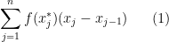
• (i) The signed definite integral , which is usually interpreted as the Riemann integral (or equivalently, the Darboux integral), which can be defined as the limit (if it exists) of the Riemann sums

  

  where is some partition of , is an element of the interval , and the limit is taken as the maximum mesh size goes to zero (this can be formalised using the concept of a net). It is convenient to adopt the convention that for ; alternatively one can interpret as the limit of the Riemann sums (1), where now the (reversed) partition goes leftwards from to , rather than rightwards from to .

• (ii) The unsigned definite integral , usually interpreted as the Lebesgue integral. The precise definition of this integral is a little complicated (see e.g. this previous post), but roughly speaking the idea is to approximate by simple functions for some coefficients and sets , and then approximate the integral by the quantities , where is the Lebesgue measure of . In contrast to the signed definite integral, no orientation is imposed or used on the underlying domain of integration, which is viewed as an “undirected” set .
• (iii) The indefinite integral or antiderivative , defined as any function whose derivative exists and is equal to on . Famously, the antiderivative is only defined up to the addition of an arbitrary constant , thus for instance .

There are some other variants of the above integrals (e.g. the Henstock-Kurzweil integral, discussed for instance in this previous post), which can handle slightly different classes of functions and have slightly different properties than the standard integrals listed here, but we will not need to discuss such alternative integrals in this course (with the exception of some improper and principal value integrals, which we will encounter in later notes).
The above three notions of integration are closely related to each other. For instance, if is a Riemann integrable function, then the signed definite integral and unsigned definite integral coincide (when the former is oriented correctly), thus

and

If is continuous, then by the fundamental theorem of calculus, it possesses an antiderivative , which is well defined up to an additive constant , and

for any , thus for instance and .
All three of the above integration concepts have analogues in complex analysis. By far the most important notion will be the complex analogue of the signed definite integral, namely the contour integral , in which the directed line segment from one real number to another is now replaced by a type of curve in the complex plane known as a contour. The contour integral can be viewed as the special case of the more general line integral , that is of particular relevance in complex analysis. There are also analogues of the Lebesgue integral, namely the arclength measure integrals and the area integrals , but these play only an auxiliary role in the subject. Finally, we still have the notion of an antiderivative (also known as a primitive) of a complex function .
As it turns out, the fundamental theorem of calculus continues to hold in the complex plane: under suitable regularity assumptions on a complex function and a primitive of that function, one has

whenever is a contour from to that lies in the domain of . In particular, functions that possess a primitive must be conservative in the sense that for any closed contour. This property of being conservative is not typical, in that “most” functions will not be conservative. However, there is a remarkable and far-reaching theorem, the Cauchy integral theorem (also known as the Cauchy-Goursat theorem), which asserts that any holomorphic function is conservative, so long as the domain is simply connected (or if one restricts attention to contractible closed contours). We will explore this theorem and several of its consequences in the next set of notes.

246A, Notes 1: complex differentiation

Previous set of notes: Notes 0. Next set of notes: Notes 2.
At the core of almost any undergraduate real analysis course are the concepts of differentiation and integration, with these two basic operations being tied together by the fundamental theorem of calculus (and its higher dimensional generalisations, such as Stokes’ theorem). Similarly, the notion of the complex derivative and the complex line integral (that is to say, the contour integral) lie at the core of any introductory complex analysis course. Once again, they are tied to each other by the fundamental theorem of calculus; but in the complex case there is a further variant of the fundamental theorem, namely Cauchy’s theorem, which endows complex differentiable functions with many important and surprising properties that are often not shared by their real differentiable counterparts. We will give complex differentiable functions another name to emphasise this extra structure, by referring to such functions as holomorphic functions. (This term is also useful to distinguish these functions from the slightly less well-behaved meromorphic functions, which we will discuss in later notes.)
In this set of notes we will focus solely on the concept of complex differentiation, deferring the discussion of contour integration to the next set of notes. To begin with, the theory of complex differentiation will greatly resemble the theory of real differentiation; the definitions look almost identical, and well known laws of differential calculus such as the product rule, quotient rule, and chain rule carry over verbatim to the complex setting, and the theory of complex power series is similarly almost identical to the theory of real power series. However, when one compares the “one-dimensional” differentiation theory of the complex numbers with the “two-dimensional” differentiation theory of two real variables, we find that the dimensional discrepancy forces complex differentiable functions to obey a real-variable constraint, namely the Cauchy-Riemann equations. These equations make complex differentiable functions substantially more “rigid” than their real-variable counterparts; they imply for instance that the imaginary part of a complex differentiable function is essentially determined (up to constants) by the real part, and vice versa. Furthermore, even when considered separately, the real and imaginary components of complex differentiable functions are forced to obey the strong constraint of being harmonic. In later notes we will see these constraints manifest themselves in integral form, particularly through Cauchy’s theorem and the closely related Cauchy integral formula.
Despite all the constraints that holomorphic functions have to obey, a surprisingly large number of the functions of a complex variable that one actually encounters in applications turn out to be holomorphic. For instance, any polynomial with complex coefficients will be holomorphic, as will the complex exponential . From this and the laws of differential calculus one can then generate many further holomorphic functions. Also, as we will show presently, complex power series will automatically be holomorphic inside their disk of convergence. On the other hand, there are certainly basic complex functions of interest that are not holomorphic, such as the complex conjugation function , the absolute value function , or the real and imaginary part functions . We will also encounter functions that are only holomorphic at some portions of the complex plane, but not on others; for instance, rational functions will be holomorphic except at those few points where the denominator vanishes, and are prime examples of the meromorphic functions mentioned previously. Later on we will also consider functions such as branches of the logarithm or square root, which will be holomorphic outside of a branch cut corresponding to the choice of branch. It is a basic but important skill in complex analysis to be able to quickly recognise which functions are holomorphic and which ones are not, as many of useful theorems available to the former (such as Cauchy’s theorem) break down spectacularly for the latter. Indeed, in my experience, one of the most common “rookie errors” that beginning complex analysis students make is the error of attempting to apply a theorem about holomorphic functions to a function that is not at all holomorphic. This stands in contrast to the situation in real analysis, in which one can often obtain correct conclusions by formally applying the laws of differential or integral calculus to functions that might not actually be differentiable or integrable in a classical sense. (This latter phenomenon, by the way, can be largely explained using the theory of distributions, as covered for instance in this previous post, but this is beyond the scope of the current course.)

Remark 1 In this set of notes it will be convenient to impose some unnecessarily generous regularity hypotheses (e.g. continuous second differentiability) on the holomorphic functions one is studying in order to make the proofs simpler. In later notes, we will discover that these hypotheses are in fact redundant, due to the phenomenon of elliptic regularity that ensures that holomorphic functions are automatically smooth.

246A, Notes 0: the complex numbers

Next set of notes: Notes 1.

Kronecker is famously reported to have said, “God created the natural numbers; all else is the work of man”. The truth of this statement (literal or otherwise) is debatable; but one can certainly view the other standard number systems as (iterated) completions of the natural numbers in various senses. For instance:

• The integers are the additive completion of the natural numbers (the minimal additive group that contains a copy of ).
• The rationals are the multiplicative completion of the integers (the minimal field that contains a copy of ).
• The reals are the metric completion of the rationals (the minimal complete metric space that contains a copy of ).
• The complex numbers are the algebraic completion of the reals (the minimal algebraically closed field that contains a copy of ).

These descriptions of the standard number systems are elegant and conceptual, but not entirely suitable for constructing the number systems in a non-circular manner from more primitive foundations. For instance, one cannot quite define the reals from scratch as the metric completion of the rationals , because the definition of a metric space itself requires the notion of the reals! (One can of course construct by other means, for instance by using Dedekind cuts or by using uniform spaces in place of metric spaces.) The definition of the complex numbers as the algebraic completion of the reals does not suffer from such a non-circularity issue, but a certain amount of field theory is required to work with this definition initially. For the purposes of quickly constructing the complex numbers, it is thus more traditional to first define as a quadratic extension of the reals , and more precisely as the extension formed by adjoining a square root of to the reals, that is to say a solution to the equation . It is not immediately obvious that this extension is in fact algebraically closed; this is the content of the famous fundamental theorem of algebra, which we will prove later in this course.
The two equivalent definitions of – as the algebraic closure, and as a quadratic extension, of the reals respectively – each reveal important features of the complex numbers in applications. Because is algebraically closed, all polynomials over the complex numbers split completely, which leads to a good spectral theory for both finite-dimensional matrices and infinite-dimensional operators; in particular, one expects to be able to diagonalise most matrices and operators. Applying this theory to constant coefficient ordinary differential equations leads to a unified theory of such solutions, in which real-variable ODE behaviour such as exponential growth or decay, polynomial growth, and sinusoidal oscillation all become aspects of a single object, the complex exponential (or more generally, the matrix exponential ). Applying this theory more generally to diagonalise arbitrary translation-invariant operators over some locally compact abelian group, one arrives at Fourier analysis, which is thus most naturally phrased in terms of complex-valued functions rather than real-valued ones. If one drops the assumption that the underlying group is abelian, one instead discovers the representation theory of unitary representations, which is simpler to study than the real-valued counterpart of orthogonal representations. For closely related reasons, the theory of complex Lie groups is simpler than that of real Lie groups.

Meanwhile, the fact that the complex numbers are a quadratic extension of the reals lets one view the complex numbers geometrically as a two-dimensional plane over the reals (the Argand plane). Whereas a point singularity in the real line disconnects that line, a point singularity in the Argand plane leaves the rest of the plane connected (although, importantly, the punctured plane is no longer simply connected). As we shall see, this fact causes singularities in complex analytic functions to be better behaved than singularities of real analytic functions, ultimately leading to the powerful residue calculus for computing complex integrals. Remarkably, this calculus, when combined with the quintessentially complex-variable technique of contour shifting, can also be used to compute some (though certainly not all) definite integrals of real-valued functions that would be much more difficult to compute by purely real-variable methods; this is a prime example of Hadamard’s famous dictum that “the shortest path between two truths in the real domain passes through the complex domain”.

Another important geometric feature of the Argand plane is the angle between two tangent vectors to a point in the plane. As it turns out, the operation of multiplication by a complex scalar preserves the magnitude and orientation of such angles; the same fact is true for any non-degenerate complex analytic mapping, as can be seen by performing a Taylor expansion to first order. This fact ties the study of complex mappings closely to that of the conformal geometry of the plane (and more generally, of two-dimensional surfaces and domains). In particular, one can use complex analytic maps to conformally transform one two-dimensional domain to another, leading among other things to the famous Riemann mapping theorem, and to the classification of Riemann surfaces.

If one Taylor expands complex analytic maps to second order rather than first order, one discovers a further important property of these maps, namely that they are harmonic. This fact makes the class of complex analytic maps extremely rigid and well behaved analytically; indeed, the entire theory of elliptic PDE now comes into play, giving useful properties such as elliptic regularity and the maximum principle. In fact, due to the magic of residue calculus and contour shifting, we already obtain these properties for maps that are merely complex differentiable rather than complex analytic, which leads to the striking fact that complex differentiable functions are automatically analytic (in contrast to the real-variable case, in which real differentiable functions can be very far from being analytic).

The geometric structure of the complex numbers (and more generally of complex manifolds and complex varieties), when combined with the algebraic closure of the complex numbers, leads to the beautiful subject of complex algebraic geometry, which motivates the much more general theory developed in modern algebraic geometry. However, we will not develop the algebraic geometry aspects of complex analysis here.

Last, but not least, because of the good behaviour of Taylor series in the complex plane, complex analysis is an excellent setting in which to manipulate various generating functions, particularly Fourier series (which can be viewed as boundary values of power (or Laurent) series ), as well as Dirichlet series . The theory of contour integration provides a very useful dictionary between the asymptotic behaviour of the sequence , and the complex analytic behaviour of the Dirichlet or Fourier series, particularly with regard to its poles and other singularities. This turns out to be a particularly handy dictionary in analytic number theory, for instance relating the distribution of the primes to the Riemann zeta function. Nowadays, many of the analytic number theory results first obtained through complex analysis (such as the prime number theorem) can also be obtained by more “real-variable” methods; however the complex-analytic viewpoint is still extremely valuable and illuminating.

We will frequently touch upon many of these connections to other fields of mathematics in these lecture notes. However, these are mostly side remarks intended to provide context, and it is certainly possible to skip most of these tangents and focus purely on the complex analysis material in these notes if desired.

Note: complex analysis is a very visual subject, and one should draw plenty of pictures while learning it. I am however not planning to put too many pictures in these notes, partly as it is somewhat inconvenient to do so on this blog from a technical perspective, but also because pictures that one draws on one’s own are likely to be far more useful to you than pictures that were supplied by someone else.

Course announcement: 246A, complex analysis

Next week, I will be teaching Math 246A, the first course in the three-quarter graduate complex analysis sequence.  This first course covers much of the same ground as an honours undergraduate complex analysis course, in particular focusing on the basic properties of holomorphic functions such as the Cauchy and residue theorems, the classification of singularities, and the maximum principle, but there will be more of an emphasis on rigour, generalisation and abstraction, and connections with other parts of mathematics.  If time permits I may also cover topics such as factorisation theorems, harmonic functions, conformal mapping, and/or applications to analytic number theory.  The main text I will be using for this course is Stein-Shakarchi (with Ahlfors as a secondary text), but as usual I will also be writing notes for the course on this blog.