Quasirandom groups and a cheap version of the Brauer-Fowler theorem

Suppose that is a finite group of even order, thus is a multiple of two. By Cauchy’s theorem, this implies that contains an involution: an element in of order two. (Indeed, if no such involution existed, then would be partitioned into doubletons together with the identity, so that would be odd, a contradiction.) Of course, groups of odd order have no involutions , thanks to Lagrange’s theorem (since cannot split into doubletons ).

The classical Brauer-Fowler theorem asserts that if a group has many involutions, then it must have a large non-trivial subgroup:

Theorem 1 (Brauer-Fowler theorem) Let be a finite group with at least involutions for some . Then contains a proper subgroup of index at most .

This theorem (which is Theorem 2F in the original paper of Brauer and Fowler, who in fact manage to sharpen slightly to ) has a number of quick corollaries which are also referred to as “the” Brauer-Fowler theorem. For instance, if is a an involution of a group , and the centraliser has order , then clearly (as contains and ) and the conjugacy class has order (since the map has preimages that are cosets of ). Every conjugate of an involution is again an involution, so by the Brauer-Fowler theorem contains a subgroup of order at least . In particular, we can conclude that every group of even order contains a proper subgroup of order at least .

Another corollary is that the size of a simple group of even order can be controlled by the size of a centraliser of one of its involutions:

Corollary 2 (Brauer-Fowler theorem) Let be a finite simple group with an involution , and suppose that has order . Then has order at most .

Indeed, by the previous discussion has a proper subgroup of index less than , which then gives a non-trivial permutation action of on the coset space . The kernel of this action is a proper normal subgroup of and is thus trivial, so the action is faithful, and the claim follows.

If one assumes the Feit-Thompson theorem that all groups of odd order are solvable, then Corollary 2 suggests a strategy (first proposed by Brauer himself in 1954) to prove the classification of finite simple groups (CFSG) by induction on the order of the group. Namely, assume for contradiction that the CFSG failed, so that there is a counterexample of minimal order to the classification. This is a non-abelian finite simple group; by the Feit-Thompson theorem, it has even order and thus has at least one involution . Take such an involution and consider its centraliser ; this is a proper subgroup of of some order . As is a minimal counterexample to the classification, one can in principle describe in terms of the CFSG by factoring the group into simple components (via a composition series) and applying the CFSG to each such component. Now, the “only” thing left to do is to verify, for each isomorphism class of , that all the possible simple groups that could have this type of group as a centraliser of an involution obey the CFSG; Corollary 2 tells us that for each such isomorphism class for , there are only finitely many that could generate this class for one of its centralisers, so this task should be doable in principle for any given isomorphism class for . That’s all one needs to do to prove the classification of finite simple groups!

Needless to say, this program turns out to be far more difficult than the above summary suggests, and the actual proof of the CFSG does not quite proceed along these lines. However, a significant portion of the argument is based on a generalisation of this strategy, in which the concept of a centraliser of an involution is replaced by the more general notion of a normaliser of a -group, and one studies not just a single normaliser but rather the entire family of such normalisers and how they interact with each other (and in particular, which normalisers of -groups commute with each other), motivated in part by the theory of Tits buildings for Lie groups which dictates a very specific type of interaction structure between these -groups in the key case when is a (sufficiently high rank) finite simple group of Lie type over a field of characteristic . See the text of Aschbacher, Lyons, Smith, and Solomon for a more detailed description of this strategy.

The Brauer-Fowler theorem can be proven by a nice application of character theory, of the type discussed in this recent blog post, ultimately based on analysing the alternating tensor power of representations; I reproduce a version of this argument (taken from this text of Isaacs) below the fold. (The original argument of Brauer and Fowler is more combinatorial in nature.) However, I wanted to record a variant of the argument that relies not on the fine properties of characters, but on the cruder theory of quasirandomness for groups, the modern study of which was initiated by Gowers, and is discussed for instance in this previous post. It gives the following slightly weaker version of Corollary 2:

Corollary 3 (Weak Brauer-Fowler theorem) Let be a finite simple group with an involution , and suppose that has order . Then can be identified with a subgroup of the unitary group .

One can get an upper bound on from this corollary using Jordan’s theorem, but the resulting bound is a bit weaker than that in Corollary 2 (and the best bounds on Jordan’s theorem require the CFSG!).

Proof: Let be the set of all involutions in , then as discussed above . We may assume that has no non-trivial unitary representation of dimension less than (since such representations are automatically faithful by the simplicity of ); thus, in the language of quasirandomness, is -quasirandom, and is also non-abelian. We have the basic convolution estimate

(see Exercise 10 from this previous blog post). In particular,

and so there are at least pairs such that , i.e. involutions whose product is also an involution. But any such involutions necessarily commute, since

Thus there are at least pairs of non-identity elements that commute, so by the pigeonhole principle there is a non-identity whose centraliser has order at least . This centraliser cannot be all of since this would make central which contradicts the non-abelian simple nature of . But then the quasiregular representation of on has dimension at most , contradicting the quasirandomness.

Mixing for progressions in non-abelian groups

I’ve just uploaded to the arXiv my paper “Mixing for progressions in non-abelian groups“, submitted to Forum of Mathematics, Sigma (which, along with sister publication Forum of Mathematics, Pi, has just opened up its online submission system). This paper is loosely related in subject topic to my two previous papers on polynomial expansion and on recurrence in quasirandom groups (with Vitaly Bergelson), although the methods here are rather different from those in those two papers. The starting motivation for this paper was a question posed in this foundational paper of Tim Gowers on quasirandom groups. In that paper, Gowers showed (among other things) that if was a quasirandom group, patterns such as were mixing in the sense that, for any four sets , the number of such quadruples in was equal to , where , and denotes a quantity that goes to zero as the quasirandomness of the group goes to infinity. In my recent paper with Vitaly, we also considered mixing properties of some other patterns, namely and . This paper is concerned instead with the pattern , that is to say a geometric progression of length three. As observed by Gowers, by applying (a suitably quantitative version of) Roth’s theorem in (cosets of) a cyclic group, one can obtain a recurrence theorem for this pattern without much effort: if is an arbitrary finite group, and is a subset of with , then there are at least pairs such that , where is a quantity depending only on . However, this argument does not settle the question of whether there is a stronger mixing property, in that the number of pairs such that should be for any . Informally, this would assert that for chosen uniformly at random from , the triplet should resemble a uniformly selected element of in some weak sense.

For non-quasirandom groups, such mixing properties can certainly fail. For instance, if is the cyclic group (which is abelian and thus highly non-quasirandom) with the additive group operation, and for some small but fixed , then in the limit , but the number of pairs with is rather than . The problem here is that the identity ensures that if and both lie in , then has a highly elevated likelihood of also falling in . One can view as the preimage of a small ball under the one-dimensional representation defined by ; similar obstructions to mixing can also be constructed from other low-dimensional representations.

However, by definition, quasirandom groups do not have low-dimensional representations, and Gowers asked whether mixing for could hold for quasirandom groups. I do not know if this is the case for arbitrary quasirandom groups, but I was able to settle the question for a specific class of quasirandom groups, namely the special linear groups over a finite field in the regime where the dimension is bounded (but is at least two) and is large. Indeed, for such groups I can obtain a count of for the number of pairs with . In fact, I have the somewhat stronger statement that there are pairs with for any .

I was also able to obtain a partial result for the length four progression in the simpler two-dimensional case , but I had to make the unusual restriction that the group element was hyperbolic in the sense that it was diagonalisable over the finite field (as opposed to diagonalisable over the algebraic closure of that field); this amounts to the discriminant of the matrix being a quadratic residue, and this holds for approximately half of the elements of . The result is then that for any , one has pairs with hyperbolic and . (Again, I actually show a slightly stronger statement in which is restricted to an arbitrary subset of hyperbolic elements.)

For the length three argument, the main tools used are the Cauchy-Schwarz inequality, the quasirandomness of , and some algebraic geometry to ensure that a certain family of probability measures on that are defined algebraically are approximately uniformly distributed. The length four argument is significantly more difficult and relies on a rather ad hoc argument involving, among other things, expander properties related to the work of Bourgain and Gamburd, and also a “twisted” version of an argument of Gowers that is used (among other things) to establish an inverse theorem for the norm.

I give some details of these arguments below the fold.

Multiple recurrence in quasirandom groups

I’ve just uploaded to the arXiv my joint paper with Vitaly Bergelson, “Multiple recurrence in quasirandom groups“, which is submitted to Geom. Func. Anal.. This paper builds upon a paper of Gowers in which he introduced the concept of a quasirandom group, and established some mixing (or recurrence) properties of such groups. A -quasirandom group is a finite group with no non-trivial unitary representations of dimension at most . We will informally refer to a “quasirandom group” as a -quasirandom group with the quasirandomness parameter large (more formally, one can work with a sequence of -quasirandom groups with going to infinity). A typical example of a quasirandom group is where is a large prime. Quasirandom groups are discussed in depth in this blog post. One of the key properties of quasirandom groups established in Gowers’ paper is the following “weak mixing” property: if are subsets of , then for “almost all” , one has

where denotes the density of in . Here, we use to informally represent an estimate of the form (where is a quantity that goes to zero when the quasirandomness parameter goes to infinity), and “almost all ” denotes “for all in a subset of of density “. As a corollary, if have positive density in (by which we mean that is bounded away from zero, uniformly in the quasirandomness parameter , and similarly for ), then (if the quasirandomness parameter is sufficiently large) we can find elements such that , , . In fact we can find approximately such pairs . To put it another way: if we choose uniformly and independently at random from , then the events , , are approximately independent (thus the random variable resembles a uniformly distributed random variable on in some weak sense). One can also express this mixing property in integral form as

for any bounded functions . (Of course, with being finite, one could replace the integrals here by finite averages if desired.) Or in probabilistic language, we have

where are drawn uniformly and independently at random from .

As observed in Gowers’ paper, one can iterate this observation to find “parallelopipeds” of any given dimension in dense subsets of . For instance, applying (1) with replaced by , , and one can assert (after some relabeling) that for chosen uniformly and independently at random from , the events , , , , , , are approximately independent whenever are dense subsets of ; thus the tuple resebles a uniformly distributed random variable in in some weak sense.

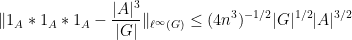
However, there are other tuples for which the above iteration argument does not seem to apply. One of the simplest tuples in this vein is the tuple in , when are drawn uniformly at random from a quasirandom group . Here, one does not expect the tuple to behave as if it were uniformly distributed in , because there is an obvious constraint connecting the last two components of this tuple: they must lie in the same conjugacy class! In particular, if is a subset of that is the union of conjugacy classes, then the events , are perfectly correlated, so that is equal to rather than . Our main result, though, is that in a quasirandom group, this is (approximately) the only constraint on the tuple. More precisely, we have

Theorem 1 Let be a -quasirandom group, and let be drawn uniformly at random from . Then for any , we have

where goes to zero as , are drawn uniformly and independently at random from , and is drawn uniformly at random from the conjugates of for each fixed choice of .

This is the probabilistic formulation of the above theorem; one can also phrase the theorem in other formulations (such as an integral formulation), and this is detailed in the paper. This theorem leads to a number of recurrence results; for instance, as a corollary of this result, we have

for almost all , and any dense subsets of ; the lower and upper bounds are sharp, with the lower bound being attained when is randomly distributed, and the upper bound when is conjugation-invariant.

To me, the more interesting thing here is not the result itself, but how it is proven. Vitaly and I were not able to find a purely finitary way to establish this mixing theorem. Instead, we had to first use the machinery of ultraproducts (as discussed in this previous post) to convert the finitary statement about a quasirandom group to an infinitary statement about a type of infinite group which we call an ultra quasirandom group (basically, an ultraproduct of increasingly quasirandom finite groups). This is analogous to how the Furstenberg correspondence principle is used to convert a finitary combinatorial problem into an infinitary ergodic theory problem.

Ultra quasirandom groups come equipped with a finite, countably additive measure known as Loeb measure , which is very analogous to the Haar measure of a compact group, except that in the case of ultra quasirandom groups one does not quite have a topological structure that would give compactness. Instead, one has a slightly weaker structure known as a -topology, which is like a topology except that open sets are only closed under countable unions rather than arbitrary ones. There are some interesting measure-theoretic and topological issues regarding the distinction between topologies and -topologies (and between Haar measure and Loeb measure), but for this post it is perhaps best to gloss over these issues and pretend that ultra quasirandom groups come with a Haar measure. One can then recast Theorem 1 as a mixing theorem for the left and right actions of the ultra approximate group on itself, which roughly speaking is the assertion that

for “almost all” , if are bounded measurable functions on , with having zero mean on all conjugacy classes of , where are the left and right translation operators

To establish this mixing theorem, we use the machinery of idempotent ultrafilters, which is a particularly useful tool for understanding the ergodic theory of actions of countable groups that need not be amenable; in the non-amenable setting the classical ergodic averages do not make much sense, but ultrafilter-based averages are still available. To oversimplify substantially, the idempotent ultrafilter arguments let one establish mixing estimates of the form (2) for “many” elements of an infinite-dimensional parallelopiped known as an IP system (provided that the actions of this IP system obey some technical mixing hypotheses, but let’s ignore that for sake of this discussion). The claim then follows by using the quasirandomness hypothesis to show that if the estimate (2) failed for a large set of , then this large set would then contain an IP system, contradicting the previous claim.

Idempotent ultrafilters are an extremely infinitary type of mathematical object (one has to use Zorn’s lemma no fewer than three times just to construct one of these objects!). So it is quite remarkable that they can be used to establish a finitary theorem such as Theorem 1, though as is often the case with such infinitary arguments, one gets absolutely no quantitative control whatsoever on the error terms appearing in that theorem. (It is also mildly amusing to note that our arguments involve the use of ultrafilters in two completely different ways: firstly in order to set up the ultraproduct that converts the finitary mixing problem to an infinitary one, and secondly to solve the infinitary mixing problem. Despite some superficial similarities, there appear to be no substantial commonalities between these two usages of ultrafilters.) There is already a fair amount of literature on using idempotent ultrafilter methods in infinitary ergodic theory, and perhaps by further development of ultraproduct correspondence principles, one can use such methods to obtain further finitary consequences (although the state of the art for idempotent ultrafilter ergodic theory has not advanced much beyond the analysis of two commuting shifts currently, which is the main reason why our arguments only handle the pattern and not more sophisticated patterns).

We also have some miscellaneous other results in the paper. It turns out that by using the triangle removal lemma from graph theory, one can obtain a recurrence result that asserts that whenever is a dense subset of a finite group (not necessarily quasirandom), then there are pairs such that all lie in . Using a hypergraph generalisation of the triangle removal lemma known as the hypergraph removal lemma, one can obtain more complicated versions of this statement; for instance, if is a dense subset of , then one can find triples such that all lie in . But the method is tailored to the specific types of patterns given here, and we do not have a general method for obtaining recurrence or mixing properties for arbitrary patterns of words in some finite alphabet such as .

We also give some properties of a model example of an ultra quasirandom group, namely the ultraproduct of where is a sequence of primes going off to infinity. Thanks to the substantial recent progress (by Helfgott, Bourgain, Gamburd, Breuillard, and others) on understanding the expansion properties of the finite groups , we have a fair amount of knowledge on the ultraproduct as well; for instance any two elements of will almost surely generate a spectral gap. We don’t have any direct application of this particular ultra quasirandom group, but it might be interesting to study it further.

254B, Notes 3: Quasirandom groups, expansion, and Selberg’s 3/16 theorem

In the previous set of notes we saw how a representation-theoretic property of groups, namely Kazhdan’s property (T), could be used to demonstrate expansion in Cayley graphs. In this set of notes we discuss a different representation-theoretic property of groups, namely quasirandomness, which is also useful for demonstrating expansion in Cayley graphs, though in a somewhat different way to property (T). For instance, whereas property (T), being qualitative in nature, is only interesting for infinite groups such as or , and only creates Cayley graphs after passing to a finite quotient, quasirandomness is a quantitative property which is directly applicable to finite groups, and is able to deduce expansion in a Cayley graph, provided that random walks in that graph are known to become sufficiently “flat” in a certain sense.

The definition of quasirandomness is easy enough to state:

Definition 1 (Quasirandom groups) Let be a finite group, and let . We say that is -quasirandom if all non-trivial unitary representations of have dimension at least . (Recall a representation is trivial if is the identity for all .)

Exercise 1 Let be a finite group, and let . A unitary representation is said to be irreducible if has no -invariant subspaces other than and . Show that is -quasirandom if and only if every non-trivial irreducible representation of has dimension at least .

Remark 1 The terminology “quasirandom group” was introduced explicitly (though with slightly different notational conventions) by Gowers in 2008 in his detailed study of the concept; the name arises because dense Cayley graphs in quasirandom groups are quasirandom graphs in the sense of Chung, Graham, and Wilson, as we shall see below. This property had already been used implicitly to construct expander graphs by Sarnak and Xue in 1991, and more recently by Gamburd in 2002 and by Bourgain and Gamburd in 2008. One can of course define quasirandomness for more general locally compact groups than the finite ones, but we will only need this concept in the finite case. (A paper of Kunze and Stein from 1960, for instance, exploits the quasirandomness properties of the locally compact group to obtain mixing estimates in that group.)

Quasirandomness behaves fairly well with respect to quotients and short exact sequences:

Exercise 2 Let be a short exact sequence of finite groups .

• (i) If is -quasirandom, show that is -quasirandom also. (Equivalently: any quotient of a -quasirandom finite group is again a -quasirandom finite group.)
• (ii) Conversely, if and are both -quasirandom, show that is -quasirandom also. (In particular, the direct or semidirect product of two -quasirandom finite groups is again a -quasirandom finite group.)

Informally, we will call quasirandom if it is -quasirandom for some “large” , though the precise meaning of “large” will depend on context. For applications to expansion in Cayley graphs, “large” will mean “ for some constant independent of the size of “, but other regimes of are certainly of interest.

The way we have set things up, the trivial group is infinitely quasirandom (i.e. it is -quasirandom for every ). This is however a degenerate case and will not be discussed further here. In the non-trivial case, a finite group can only be quasirandom if it is large and has no large subgroups:

Exercise 3 Let , and let be a finite -quasirandom group.

• (i) Show that if is non-trivial, then . (Hint: use the mean zero component of the regular representation .) In particular, non-trivial finite groups cannot be infinitely quasirandom.
• (ii) Show that any proper subgroup of has index . (Hint: use the mean zero component of the quasiregular representation.)

The following exercise shows that quasirandom groups have to be quite non-abelian, and in particular perfect:

Exercise 4 (Quasirandomness, abelianness, and perfection) Let be a finite group.

• (i) If is abelian and non-trivial, show that is not -quasirandom. (Hint: use Fourier analysis or the classification of finite abelian groups.)
• (ii) Show that is -quasirandom if and only if it is perfect, i.e. the commutator group is equal to . (Equivalently, is -quasirandom if and only if it has no non-trivial abelian quotients.)

Later on we shall see that there is a converse to the above two exercises; any non-trivial perfect finite group with no large subgroups will be quasirandom.

Exercise 5 Let be a finite -quasirandom group. Show that for any subgroup of , is -quasirandom, where is the index of in . (Hint: use induced representations.)

Now we give an example of a more quasirandom group.

Lemma 2 (Frobenius lemma) If is a field of some prime order , then is -quasirandom.

This should be compared with the cardinality of the special linear group, which is easily computed to be .

Proof: We may of course take to be odd. Suppose for contradiction that we have a non-trivial representation on a unitary group of some dimension with . Set to be the group element

and suppose first that is non-trivial. Since , we have ; thus all the eigenvalues of are roots of unity. On the other hand, by conjugating by diagonal matrices in , we see that is conjugate to (and hence conjugate to ) whenever is a quadratic residue mod . As such, the eigenvalues of must be permuted by the operation for any quadratic residue mod . Since has at least one non-trivial eigenvalue, and there are distinct quadratic residues, we conclude that has at least distinct eigenvalues. But is a matrix with , a contradiction. Thus lies in the kernel of . By conjugation, we then see that this kernel contains all unipotent matrices. But these matrices generate (see exercise below), and so is trivial, a contradiction.

Exercise 6 Show that for any prime , the unipotent matrices

for ranging over generate as a group.

Exercise 7 Let be a finite group, and let . If is generated by a collection of -quasirandom subgroups, show that is itself -quasirandom.

Exercise 8 Show that is -quasirandom for any and any prime . (This is not sharp; the optimal bound here is , which follows from the results of Landazuri and Seitz.)

As a corollary of the above results and Exercise 2, we see that the projective special linear group is also -quasirandom.

Remark 2 One can ask whether the bound in Lemma 2 is sharp, assuming of course that is odd. Noting that acts linearly on the plane , we see that it also acts projectively on the projective line , which has elements. Thus acts via the quasiregular representation on the -dimensional space , and also on the -dimensional subspace ; this latter representation (known as the Steinberg representation) is irreducible. This shows that the bound cannot be improved beyond . More generally, given any character , acts on the -dimensional space of functions that obey the twisted dilation invariance for all and ; these are known as the principal series representations. When is the trivial character, this is the quasiregular representation discussed earlier. For most other characters, this is an irreducible representation, but it turns out that when is the quadratic representation (thus taking values in while being non-trivial), the principal series representation splits into the direct sum of two -dimensional representations, which comes very close to matching the bound in Lemma 2. There is a parallel series of representations to the principal series (known as the discrete series) which is more complicated to describe (roughly speaking, one has to embed in a quadratic extension and then use a rotated version of the above construction, to change a split torus into a non-split torus), but can generate irreducible representations of dimension , showing that the bound in Lemma 2 is in fact exactly sharp. These constructions can be generalised to arbitrary finite groups of Lie type using Deligne-Luzstig theory, but this is beyond the scope of this course (and of my own knowledge in the subject).

Exercise 9 Let be an odd prime. Show that for any , the alternating group is -quasirandom. (Hint: show that all cycles of order in are conjugate to each other in (and not just in ); in particular, a cycle is conjugate to its power for all . Also, as , is simple, and so the cycles of order generate the entire group.)

Remark 3 By using more precise information on the representations of the alternating group (using the theory of Specht modules and Young tableaux), one can show the slightly sharper statement that is -quasirandom for (but is only -quasirandom for due to icosahedral symmetry, and -quasirandom for due to lack of perfectness). Using Exercise 3 with the index subgroup , we see that the bound cannot be improved. Thus, (for large ) is not as quasirandom as the special linear groups (for large and bounded), because in the latter case the quasirandomness is as strong as a power of the size of the group, whereas in the former case it is only logarithmic in size.

If one replaces the alternating group with the slightly larger symmetric group , then quasirandomness is destroyed (since , having the abelian quotient , is not perfect); indeed, is -quasirandom and no better.

Remark 4 Thanks to the monumental achievement of the classification of finite simple groups, we know that apart from a finite number (26, to be precise) of sporadic exceptions, all finite simple groups (up to isomorphism) are either a cyclic group , an alternating group , or is a finite simple group of Lie type such as . (We will define the concept of a finite simple group of Lie type more precisely in later notes, but suffice to say for now that such groups are constructed from reductive algebraic groups, for instance is constructed from in characteristic .) In the case of finite simple groups of Lie type with bounded rank , it is known from the work of Landazuri and Seitz that such groups are -quasirandom for some depending only on the rank. On the other hand, by the previous remark, the large alternating groups do not have this property, and one can show that the finite simple groups of Lie type with large rank also do not have this property. Thus, we see using the classification that if a finite simple group is -quasirandom for some and is sufficiently large depending on , then is a finite simple group of Lie type with rank . It would be of interest to see if there was an alternate way to establish this fact that did not rely on the classification, as it may lead to an alternate approach to proving the classification (or perhaps a weakened version thereof).

A key reason why quasirandomness is desirable for the purposes of demonstrating expansion is that quasirandom groups happen to be rapidly mixing at large scales, as we shall see below the fold. As such, quasirandomness is an important tool for demonstrating expansion in Cayley graphs, though because expansion is a phenomenon that must hold at all scales, one needs to supplement quasirandomness with some additional input that creates mixing at small or medium scales also before one can deduce expansion. As an example of this technique of combining quasirandomness with mixing at small and medium scales, we present a proof (due to Sarnak-Xue, and simplified by Gamburd) of a weak version of the famous “3/16 theorem” of Selberg on the least non-trivial eigenvalue of the Laplacian on a modular curve, which among other things can be used to construct a family of expander Cayley graphs in (compare this with the property (T)-based methods in the previous notes, which could construct expander Cayley graphs in for any fixed ).