A (smooth) Riemannian manifold is a smooth manifold  without boundary, equipped with a Riemannian metric
  , which assigns a length
  to every tangent vector
  at a point
  , and more generally assigns an inner product

to every pair of tangent vectors  at a point . (We use Roman font for
  here, as we will need to use to denote group elements later in this post.) This inner product is assumed to symmetric, positive definite, and smoothly varying in
  , and the length is then given in terms of the inner product by the formula

In coordinates (and also using abstract index notation), the metric can be viewed as an invertible symmetric rank  tensor
  , with

One can also view the Riemannian metric as providing a (self-adjoint) identification between the tangent bundle  of the manifold and the cotangent bundle
  ; indeed, every tangent vector is then identified with the cotangent vector
  , defined by the formula

In coordinates,  .
.
A fundamental dynamical system on the tangent bundle (or equivalently, the cotangent bundle, using the above identification) of a Riemannian manifold is that of geodesic flow. Recall that geodesics are smooth curves ![{\gamma: [a,b] \rightarrow M}](https://s0.wp.com/latex.php?latex=%7B%5Cgamma%3A+%5Ba%2Cb%5D+%5Crightarrow+M%7D&bg=ffffff&fg=000000&s=0&c=20201002) that minimise the length
that minimise the length

There is some degeneracy in this definition, because one can reparameterise the curve  without affecting the length. In order to fix this degeneracy (and also because the square of the speed is a more tractable quantity analytically than the speed itself), it is better if one replaces the length with the energy

Minimising the energy of a parameterised curve turns out to be the same as minimising the length, together with an additional requirement that the speed  stay constant in time. Minimisers (and more generally, critical points) of the energy functional (holding the endpoints fixed) are known as geodesic flows. From a physical perspective, geodesic flow governs the motion of a particle that is subject to no external forces and thus moves freely, save for the constraint that it must always lie on the manifold .
One can also view geodesic flows as a dynamical system on the tangent bundle (with the state at any time  given by the position
  and the velocity
  ) or on the cotangent bundle (with the state then given by the position and the momentum
  ). With the latter perspective (sometimes referred to as cogeodesic flow), geodesic flow becomes a Hamiltonian flow, with Hamiltonian
  given as

where  is the inverse inner product to
  , which can be defined for instance by the formula

In coordinates, geodesic flow is given by Hamilton’s equations of motion

In terms of the velocity  , we can rewrite these equations as the geodesic equation

where

are the Christoffel symbols; using the Levi-Civita connection  , this can be written more succinctly as

If the manifold is an embedded submanifold of a larger Euclidean space  , with the metric on being induced from the standard metric on
  , then the geodesic flow equation can be rewritten in the equivalent form

where is now viewed as taking values in , and  is similarly viewed as a subspace of . This is intuitively obvious from the geometric interpretation of geodesics: if the curvature of a curve contains components that are transverse to the manifold rather than normal to it, then it is geometrically clear that one should be able to shorten the curve by shifting it along the indicated transverse direction. It is an instructive exercise to rigorously formulate the above intuitive argument. This fact also conforms well with one’s physical intuition of geodesic flow as the motion of a free particle constrained to be in ; the normal quantity
  then corresponds to the centripetal force necessary to keep the particle lying in (otherwise it would fly off along a tangent line to , as per Newton’s first law). The precise value of the normal vector can be computed via the second fundamental form as
  , but we will not need this formula here.
In a beautiful paper from 1966, Vladimir Arnold (who, sadly, passed away last week), observed that many basic equations in physics, including the Euler equations of motion of a rigid body, and also (by which is a priori a remarkable coincidence) the Euler equations of fluid dynamics of an inviscid incompressible fluid, can be viewed (formally, at least) as geodesic flows on a (finite or infinite dimensional) Riemannian manifold. And not just any Riemannian manifold: the manifold is a Lie group (or, to be truly pedantic, a torsor of that group), equipped with a right-invariant (or left-invariant, depending on one’s conventions) metric. In the context of rigid bodies, the Lie group is the group  of rigid motions; in the context of incompressible fluids, it is the group
  ) of measure-preserving diffeomorphisms. The right-invariance makes the Hamiltonian mechanics of geodesic flow in this context (where it is sometimes known as the Euler-Arnold equation or the Euler-Poisson equation) quite special; it becomes (formally, at least) completely integrable, and also indicates (in principle, at least) a way to reformulate these equations in a Lax pair formulation. And indeed, many further completely integrable equations, such as the Korteweg-de Vries equation, have since been reinterpreted as Euler-Arnold flows.
From a physical perspective, this all fits well with the interpretation of geodesic flow as the free motion of a system subject only to a physical constraint, such as rigidity or incompressibility. (I do not know, though, of a similarly intuitive explanation as to why the Korteweg de Vries equation is a geodesic flow.)
One consequence of being a completely integrable system is that one has a large number of conserved quantities. In the case of the Euler equations of motion of a rigid body, the conserved quantities are the linear and angular momentum (as observed in an external reference frame, rather than the frame of the object). In the case of the two-dimensional Euler equations, the conserved quantities are the pointwise values of the vorticity (as viewed in Lagrangian coordinates, rather than Eulerian coordinates). In higher dimensions, the conserved quantity is now the (Hodge star of) the vorticity, again viewed in Lagrangian coordinates. The vorticity itself then evolves by the vorticity equation, and is subject to vortex stretching as the diffeomorphism between the initial and final state becomes increasingly sheared.
The elegant Euler-Arnold formalism is reasonably well-known in some circles (particularly in Lagrangian and symplectic dynamics, where it can be viewed as a special case of the Euler-Poincaré formalism or Lie-Poisson formalism respectively), but not in others; I for instance was only vaguely aware of it until recently, and I think that even in fluid mechanics this perspective to the subject is not always emphasised. Given the circumstances, I thought it would therefore be appropriate to present Arnold’s original 1966 paper here. (For a more modern treatment of these topics, see the books of Arnold-Khesin and Marsden-Ratiu.)
In order to avoid technical issues, I will work formally, ignoring questions of regularity or integrability, and pretending that infinite-dimensional manifolds behave in exactly the same way as their finite-dimensional counterparts. In the finite-dimensional setting, it is not difficult to make all of the formal discussion below rigorous; but the situation in infinite dimensions is substantially more delicate. (Indeed, it is a notorious open problem whether the Euler equations for incompressible fluids even forms a global continuous flow in a reasonable topology in the first place!) However, I do not want to discuss these analytic issues here; see this paper of Ebin and Marsden for a treatment of these topics.
— 1. Geodesic flow using a right-invariant metric —
Let  be a Lie group. From a physical perspective, one should think of a group element as describing the relationship between a fixed reference observer
  , and a moving object
  ; mathematically, one could think of
  and as belonging to a (left) torsor of . (One could also work with right torsors; this would require a number of sign conventions below to be altered.) For instance, in the case of rigid motions, would be the reference state of a rigid body, would be the current state, and
  would be the element of the rigid motion group that moves to ; is then the configuration space of the rigid body. Similarly, in the case of incompressible fluids, would be a reference state of the fluid (e.g. the initial state at time
  ), would be the current state, and
  would be the measure-preserving diffeomorphism required to map the location each particle of the fluid at to the corresponding location of the same particle at . Again, would be the configuration space of the fluid.
Once one fixes the reference observer , one can set up a bijection between the torsor and the group ; but one can also adopt a “coordinate-free” perspective in which the observer is not present, in which case one should keep and distinct. Strictly speaking, the geodesic flow we will introduce will be on rather than on , but for some minor notational reasons it is convenient to fix a reference observer in order to identify the two objects.
Let  denote the Lie algebra of , i.e. the tangent space of at the identity. This Lie algebra can be identified with the tangent space
  of a state in in two different ways: an intrinsic one that does not use a reference observer , and an extrinsic one which does rely on this observer.
- (Intrinsic identification) If
 is a tangent vector to , we let
  be the associated element of the Lie algebra defined infinitesimally as

modulo higher order terms for infinitesimal  , or more traditionally by requiring
  whenever
  ,
,  are smooth curves such that
  . Conversely, if
  , we let
  be the tangent vector at defined infinitesimally as

modulo higher order terms for infinitesimal , or more traditionally by requiring  whenever , are smooth curves such that (so
  ). Clearly, these two operations invert each other.
- (Extrinsic identification) If is a tangent vector to , and
 for some fixed reference , we let
  be the element of the Lie algebra defined infinitesimally as

or more traditionally by requiring  whenever ,
  are such that
  and
and  .
.
The distinction between intrinsic and extrinsic identifications is closely related to the distinction between active and passive transformations:  denotes the direction in which must move in order to effect a change of
  in the apparent position of relative to any observer , whereas
  is the (inverse of the) direction in which the reference would move to effect the same change in the apparent position. The two quantities are related to each other by conjugation:

where we define conjugation  of a Lie algebra element
  by a Lie group element in the usual manner.
If  is the state of a rigid body at time , then
  is the linear and angular velocity of
  as measured in ‘s current spatial reference frame, while if
  , then
  is the linear and angular velocity of as measured in the frame of . Similarly, if is the state of an incompressible fluid at time , then is the velocity field
  in Eulerian coordinates, while is the velocity field
  in Lagrangian coordinates.
The left action of  on the torsor induces a corresponding action
  on the tangent bundle . Indeed, this action was implicitly present in the notation used earlier.
Now suppose we choose a non-degenerate inner product  on the Lie algebra
  . We do not assume any symmetries or invariances of this inner product with respect to the group structure, such as conjugation invariance; in particular, this inner product will usually not be the Cartan-Killing form. At any rate, once we select an inner product, we can construct a right-invariant Riemannian metric on by the formula

Because we do not require the inner product to be conjugation invariant, this metric will usually not be bi-invariant, instead being merely right-invariant.
The quantity  is the Hamiltonian associated to this metric. For rigid bodies, this Hamiltonian is the total kinetic energy of the body, which is the sum of the kinetic energy
  of the centre of mass, plus the rotational kinetic energy
  which is determined by the moments of inertia
  . For incompressible fluids, the Hamiltonian is (up to a normalising constant) the energy
  of the fluid, which can be computed either in Eulerian coordinates or in Lagrangian coordinates (there are no Jacobian factors here thanks to incompressibility).
Another important object in the Euler-Arnold formalism is the bilinear form  associated to the inner product
  , defined via the Lie bracket and duality using the formula
![\displaystyle \langle [X,Y], Z \rangle = \langle B(Z,Y), X \rangle, \ \ \ \ \ (2)](https://s0.wp.com/latex.php?latex=%5Cdisplaystyle++%5Clangle+%5BX%2CY%5D%2C+Z+%5Crangle+%3D+%5Clangle+B%28Z%2CY%29%2C+X+%5Crangle%2C+%5C+%5C+%5C+%5C+%5C+%282%29&bg=ffffff&fg=000000&s=0&c=20201002)
thus  is a partial adjoint of the Lie bracket operator. (The conventions here differ slightly from those in Arnold’s paper.) Note that this form need not be symmetric. The importance of this form comes from the fact that it describes the geodesic flow:
Theorem 1 (Euler-Arnold equation) Let be a geodesic flow on using the right-invariant metric defined above, and let  be the intrinsic velocity vector. Then obeys the equation

The Euler-Arnold equation is also known as the Euler-Poincaré equation; see for instance this paper of Cendra, Marsden, Pekarsky, and Ratiu for further discussion.
Proof: For notational reasons, we will prove this in the model case when is a matrix group (so that we can place , , and in a common vector space, or more precisely a common matrix space); the general case is similar but requires more abstract notation. We consider a variation  of the original curve
  , and consider the first variation of the energy

which we write using (1) as

We move the derivative inside and use symmetry to write this as

or
We expand

Similarly

and thus
![\displaystyle \partial_s(\gamma_t \gamma^{-1}) = \partial_t(\gamma_s \gamma^{-1}) + [\gamma_s \gamma^{-1}, X ].](https://s0.wp.com/latex.php?latex=%5Cdisplaystyle+%5Cpartial_s%28%5Cgamma_t+%5Cgamma%5E%7B-1%7D%29+%3D+%5Cpartial_t%28%5Cgamma_s+%5Cgamma%5E%7B-1%7D%29+%2B+%5B%5Cgamma_s+%5Cgamma%5E%7B-1%7D%2C+X+%5D.&bg=ffffff&fg=000000&s=0&c=20201002)
Inserting this into the first variation and integrating by parts, we obtain
![\displaystyle \int_a^b \langle [\gamma_s \gamma^{-1}, X], X \rangle - \langle \gamma_s \gamma^{-1}, \partial_t X \rangle\ dt;](https://s0.wp.com/latex.php?latex=%5Cdisplaystyle++%5Cint_a%5Eb+%5Clangle+%5B%5Cgamma_s+%5Cgamma%5E%7B-1%7D%2C+X%5D%2C+X+%5Crangle+-+%5Clangle+%5Cgamma_s+%5Cgamma%5E%7B-1%7D%2C+%5Cpartial_t+X+%5Crangle%5C+dt%3B&bg=ffffff&fg=000000&s=0&c=20201002)
using (2), this is

and so the first variation vanishes for arbitrary choices of perturbation  precisely when
  , as required.
It is instructive to verify that the Hamiltonian  is preserved by this equation, as it should be. In the case of rigid motions, (3) is essentially Euler’s equations of motion.
The right-invariance of the Riemannian manifold implies that the geodesic flow is similarly right-invariant. And this is reflected by the fact that the Euler-Arnold equation (3) does not involve the position  . This position of course evolves by the equation

which is just the definition of .
Note that while the velocity influences the evolution of the position , the position does not influence the evolution of the velocity . This is of course a manifestation of the right-invariance of the problem. This reduction of the flow is known as Euler-Poincaré reduction, and is essentially a basic example of both Lagrangian reduction and symplectic reduction, in which the symmetries of a Lagrangian or Hamiltonian evolution are used to reduce the dimension of the dynamics while preserving the Lagrangian or Hamiltonian structure.
We can rephrase the Euler equation in a Lax pair formulation by introducing the Cartan-Killing form

Like , the Cartan-Killing form  is a symmetric bilinear form on the Lie algebra . If we assume that the group is semisimple (and finite-dimensional), then this form will be non-degenerate. It obeys the identity
![\displaystyle ([X,Y],Z) = -(Y,[X,Z]), \ \ \ \ \ (5)](https://s0.wp.com/latex.php?latex=%5Cdisplaystyle++%28%5BX%2CY%5D%2CZ%29+%3D+-%28Y%2C%5BX%2CZ%5D%29%2C+%5C+%5C+%5C+%5C+%5C+%285%29&bg=ffffff&fg=000000&s=0&c=20201002)
thus adjoints are automatically skew-adjoint in the Cartan-Killing form.
If the Cartan-Killing form is non-degenerate, it can be used to express the inner product via a formula of the form

where  is an invertible linear transformation which is self-adjoint with respect to both
  and . We then define the intrinsic momentum
  of the Euler-Arnold flow by the formula

From (3), we see that  evolves by the equation
But observe from (6), (2), (6), (5) that

![\displaystyle = \langle [Y, \Lambda {\bf M}], \Lambda {\bf M} \rangle](https://s0.wp.com/latex.php?latex=%5Cdisplaystyle++%3D+%5Clangle+%5BY%2C+%5CLambda+%7B%5Cbf+M%7D%5D%2C+%5CLambda+%7B%5Cbf+M%7D+%5Crangle&bg=ffffff&fg=000000&s=0&c=20201002)
![\displaystyle = ([Y,\Lambda {\bf M}], {\bf M} )](https://s0.wp.com/latex.php?latex=%5Cdisplaystyle++%3D+%28%5BY%2C%5CLambda+%7B%5Cbf+M%7D%5D%2C+%7B%5Cbf+M%7D+%29&bg=ffffff&fg=000000&s=0&c=20201002)
![\displaystyle = ([\Lambda {\bf M},{\bf M}],Y)](https://s0.wp.com/latex.php?latex=%5Cdisplaystyle++%3D+%28%5B%5CLambda+%7B%5Cbf+M%7D%2C%7B%5Cbf+M%7D%5D%2CY%29+&bg=ffffff&fg=000000&s=0&c=20201002)
for any test vector  , which by nondegeneracy implies that
![\displaystyle \Lambda^{-1} B( \Lambda {\bf M}, \Lambda {\bf M} ) = [\Lambda {\bf M},{\bf M}]](https://s0.wp.com/latex.php?latex=%5Cdisplaystyle+%5CLambda%5E%7B-1%7D+B%28+%5CLambda+%7B%5Cbf+M%7D%2C+%5CLambda+%7B%5Cbf+M%7D+%29+%3D+%5B%5CLambda+%7B%5Cbf+M%7D%2C%7B%5Cbf+M%7D%5D&bg=ffffff&fg=000000&s=0&c=20201002)
leading to the Lax pair form
![\displaystyle \frac{d}{dt} {\bf M} = [\Lambda {\bf M},{\bf M}]](https://s0.wp.com/latex.php?latex=%5Cdisplaystyle++%5Cfrac%7Bd%7D%7Bdt%7D+%7B%5Cbf+M%7D+%3D+%5B%5CLambda+%7B%5Cbf+M%7D%2C%7B%5Cbf+M%7D%5D&bg=ffffff&fg=000000&s=0&c=20201002)
of the Euler-Arnold equation, known as the Lie-Poisson equation. (The sign conventions here are the opposite of those in Arnold’s paper, I think ultimately because I am assuming right-invariance instead of left-invariance.) In particular, the spectrum of is invariant, or equivalently evolves along a single coadjoint orbit in  .
.
By Noether’s theorem, the right-invariance of the geodesic flow should create a conserved quantity (or moment map); as the right-invariance is an action of the group , the conserved quantity should take place in the adjoint  . If we write
  for some fixed observer , then this conserved quantity can be computed as the extrinsic momentum

thus  is the
  -form associated to , pulled back to extrinsic coordinates. Indeed, from (4) one has

and thus
and hence for any test vector 
![\displaystyle \partial_t P(Y) = \langle X_t, g Y g^{-1} \rangle + \langle X, [X, gYg^{-1}] \rangle](https://s0.wp.com/latex.php?latex=%5Cdisplaystyle++%5Cpartial_t+P%28Y%29+%3D+%5Clangle+X_t%2C+g+Y+g%5E%7B-1%7D+%5Crangle+%2B+%5Clangle+X%2C+%5BX%2C+gYg%5E%7B-1%7D%5D+%5Crangle&bg=ffffff&fg=000000&s=0&c=20201002)


thanks to (2), and the claim follows. Using the Cartan-Killing form, the extrinsic momentum can also be identified with  , thus linking the extrinsic and intrinsic momenta to each other.
— 2. Incompressible fluids —
Now consider an incompressible fluid in  , whose initial state is and whose state at any time is given as . One can express , where
  is the diffeomorphism from to itself that maps the location of each particle at to the location of the same particle at . As the fluid is assumed incompressible, the diffeomorphism must be measure-preserving (and orientation preserving); we denote the group of such special diffeomorphisms as
  .
.
The Lie algebra to the group  of all diffeomorphisms, is the space of all (smooth) vector fields
  . The Lie algebra of the subgroup of measure-preserving diffeomorphisms is the space of all divergence-free vector fields; indeed, this is one of the primary motivations of introducing the concept of divergence of a vector field. We give both Lie algebras the usual
  inner product:

The Lie bracket on or is the same as the usual Lie bracket of vector fields.
Let  be the intrinsic velocity vector; then this is a divergence-free vector field, which physically represents the velocity field in Eulerian coordinates. The extrinsic velocity vector
 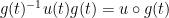 is then the velocity field in Lagrangian coordinates; it is also divergence-free.
If there were no constraint of incompressibility (i.e. if one were working in rather than ), then the metric is flat, and the geodesic equation of motion is simply given by Newton’s first law

or in terms of the intrinsic velocity field  ,
,
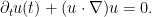
Once we restrict to incompressible fluids, this becomes

or, in terms of the intrinsic velocity field,

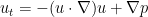
or equivalently (by Hodge theory)
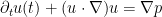
for some  ; this is precisely the Euler equations of incompressible fluids. This equation can also be deduced from (3), after first calculating using (2) and the formula for Lie bracket of vector fields that
  is the divergence-free component of
  ; we omit the details (which are in Arnold’s paper).
Let us now compute the extrinsic momentum  , which is conserved by the Euler equations. Given any divergence-free vector field
  (in Lagrangian coordinates), we see from (7) that is given by the formula

thus the form  is computed by pushing over to Eulerian coordinates to get
  and then taking the inner product with . Let us check that this is indeed conserved. Since
and

where  denotes the Lie derivative along the vector field , we see that

where  is in Eulerian coordinates. The
  term vanishes by integration by parts, since (and hence
  ) is divergence-free. The Lie derivative is computed by the formula

As  is a total derivative (recall here that is divergence-free), this term vanishes. The other two terms combine to form a total derivative
  , which also vanishes, and so the claim follows.
The external momentum is closely related to the vorticity  . This is because a divergence-free vector field can (in principle, at least) be written as the divergence
  of a
of a  -vector field
  . As divergence is diffeomorphism invariant, it commutes with pushforward:

and thus


where  is the Hodge star. We can pull this back to Lagrangian coordinates to obtain
As was an arbitrary -form, we thus see that the pullback  of the Hodge star of the vorticity in Lagrangian coordinates is preserved by the flow, or equivalently that
  is transported by the velocity field . In the two-dimensional case, this is well known ( is a scalar in this case); in higher dimensions, this is fact is implicit in the vorticity equation

which can be rewritten as

In principle, the Euler-Arnold formalism allows one to write the Euler equations for incompressible fluids into a Lax pair form. To properly carry this out by the machinery above, though, would require calculating the Cartan-Killing form for the infinite-dimensional Lie group , which looked quite tricky to me, and I was not able to complete the calculation. However, a Lax pair formulation for this system was found by Friedlander and Vishik, and it is likely that that formulation is essentially equivalent to the Lax pair that one could construct from the Euler-Arnold formalism. In the simpler two-dimensional case, it was observed by Li that the vorticity equation can also be recast into a slightly different Lax pair form. While this formalism does allow for some of the inverse scattering machinery to be brought to bear on the initial value problem for the Euler equations, it does not as yet seem that this machinery can be successfully used for the global regularity problem.
It would, of course, also be very interesting to see what aspects of this formalism carry over to the Navier-Stokes equation. The first naive guess would be to add a friction term, but this seems to basically correspond to adding a damping factor of  (rather than a viscosity factor of
  ) to the Euler equations and ends up being rather uninteresting (it basically slows down the time variable but otherwise does not affect the dynamics). More generally, it would be of interest to see how the Hamiltonian formalism can be generalised to incorporate dissipation or viscosity.
{\emph Update}, June 15: Some references added. Thanks to Jerry Marsden for comments.


31 comments
Comments feed for this article
8 June, 2010 at 12:45 am
Igor Carron
Terry,
Typo in LaTeX ?
“..we let [Formula does not parse] be the tangent vector at A defined infinitesimally…”
Igor.
[This seemed to be a transient problem with WordPress’s LaTeX image rendering server; it disappeared by the time I got around to looking at it. -T.]
8 June, 2010 at 6:37 am
David Corfield
Extra ‘to’ in “…a system subject to only to a physical constraint…”.
Section 3 of Hydrodynamics and Infinite-Dimensional Riemannian Geometry gives some insight as to the KdV equation as geodesic flow, but not so straightforwardly as the free motion of a system subject only to a physical constraint.
[Corrected, and thanks for the link! – T.]
8 June, 2010 at 6:48 pm
Christian
There is some interesting recent work by Holm on co-workers on dissipative systems which are still co-adjoint, see for example http://rspa.royalsocietypublishing.org/content/early/2010/04/21/rspa.2010.0043.abstract. They consider kinetic theory, and hence $Diff_{can}$, but the approach using double Poisson brackets is also applicable to fluid systems, see the earlier article by Bloch et al; http://infoscience.epfl.ch/record/129486.
9 June, 2010 at 3:38 am
HB
Minor typo (second equation):
“… the length is then given in terms of the inner product by the formula”
|v|^2:=
^2 is missing.
[Corrected, thanks – T.]
9 June, 2010 at 5:44 am
John Sidles
Thank you for this fine post, and especially for its tribute to Vladimir Arnold. I am hoping that someday you may write a post that discusses the extension of these geometric/dynamical ideas to the quantum domain, where many of them carry-over without change … and some of them become simpler. Arnold discusses these quantum extensions in (too brief!) Appendix 3 of his Mathematical Methods of Classical Mechanics, but nowadays we appreciate that there is much more to be said.
Nowadays, in quantum systems engineering, the natural pullback is not from (say) classical Cartesian space onto the manifold of rigid body rotations and translations, but from Hilbert space onto the manifold of tensor network states. Just as dissipation and viscosity play central roles in classical systems, Lindbladian dynamics plays a key role in quantum dynamics. And in all of the preceding, the natural pullback of dynamics onto reduced-dimension manifolds is central to achieving a satisfactory mathematical, physical, and engineering understanding.
One challenge that the mathematical, physical science, and engineering communities are all facing is that (typically) our students do not acquire (as undergraduates at least) a mathematically natural toolset for appreciating these ubiquitous “Arnoldian” ideas.
Learning these ideas at the graduate level is not particularly satisfactory either, in that specialization sets-in to a degree that inhibits graduate students in math, physics, chemistry, biology, mechatronics, materials science (etc.) from appreciating that they are all embracing the same “Arnoldian” ideas, but speaking very different languages. Too often, moreover, these languages are not mathematically natural in the sense that Arnold so scrupulously respect.
It is easy to write a long wish-list of “Arnoldian” topics that mathematicians might beneficially explain in ways that are accessible to engineers and scientists. To name two, I wish someone would explain Ran Raz’ STOC2010 presentation Tensor-Rank and Lower Bounds for Arithmetic Formulas, which appears to lie at the boundary of complexity theory, algebraic geometry, and quantum simulation theory … but I have to confess to being (so far) unable to decode Raz’ article itself. And I wish someone would tackle the “Arnoldian” analysis of Lindblad processes. The standard textbooks analyze these processes using vector-space proof technology, but we engineers use these processes in an “Arnoldian” pullback context (for which much of the vector-space toolset is inapplicable); this leaves us engineers with sadly little geometric and/or informatic insight into our own simulation codes.
That being said, I am *very* grateful for the existence of this fine weblog—and for many other outstanding math weblogs too—which so greatly encourage us engineers and scientists, by allowing us to glimpse the many wonderful “Arnoldian” opportunities, both creative and practical, that are open to us all.
9 June, 2010 at 7:35 am
Peter
It looks like there’s a typo in the definition of the Christoffel symbol – the first two terms in the parenthesis are the same.
[Corrected, thanks – T.]
9 June, 2010 at 11:36 am
Michael Nielsen
A connection I’m very fond of is between quantum computing and minimal geodesic paths on right-invariant manifolds. It can be shown that the minimal quantum circuit size for solving a particular problem is equal (modulo polynomial factors and some technical caveats) to the minimal geodesic length between two points on a particular right-invariant manifold.
This seems to me a potentially very useful observation for understanding minimal circuit sizes. Pretty much everything we teach students about minimizing functions relies on working in a smooth space, where the tools of calculus can be used. Unfortunately, the way we ordinarily think about circuits (quantum and non-quantum) that way of thinking can’t be applied to understand minimal circuit size. But by relating circuit size to geometry it becomes possible to use the tools of calculus to think about minimal circuit complexity. Roughly, there’s a correspondence optimal quantum circuit to solve a particular problem and some solution of the Euler-Arnold equation. This seems like a potentially powerful observation, although I was never able to get bounds on circuit size this way. I wrote up some of these ideas in http://arxiv.org/abs/quant-ph/0701004 (joint with Mark Dowling), if anyone’s interested.
23 June, 2010 at 8:09 pm
Chirag Lakhani
Dear Michael,
I know I have come to this post late, but I was wondering if you think there is any advantage if formulating your ideas in terms of this symplectic geometry setting rather than Riemannian geometry. Do things like Euler-Poison reduction work out when it comes to the metric you use for SU(2^n)?
24 June, 2010 at 6:57 am
Michael Nielsen
I didn’t consider this at all – it certainly seems an interesting question. My background in symplectic geometry is minimal.
10 June, 2010 at 8:23 am
Anosh Joseph
Great post, Terry. Here is a recent review on this in a recent arXiv paper :
http://arxiv.org/abs/0906.0184
10 June, 2010 at 11:38 am
John Sidles
Anosh, thank you for that arXiv reference … which was new to me and fun. Perhaps you might similarly enjoy astronaut Michael Foale’s keynote address “Navigating on Mir” (which was published in Mathematica Journal) in which the negative sectional curvature of rigid-body state-space generates high adventure in low Earth orbit.
The fraction of the Earth’s global computing power that is devoted to numerically integrating rigid-body rotational dynamics is surprising large … plausibly as large as 10^(-4)—10(^-3) … for the reason that tumbling water molecules are ubiquitously present in molecular dynamical simulations.
Moreover, for reasons of numerical efficiency, water-molecule dynamical trajectories typically are integrated on quaternionic state-spaces; thus yet another of this blog’s perennial mathematical themes appears naturally … gauge invariance!
16 June, 2010 at 7:08 am
Vladimir Arnold (1937-2010). R.I.P. « Successful Researcher
[…] Vladimir Arnold (1937-2010). R.I.P. One of the world’s greatest and most influential mathematicians, Vladimir Arnold, passed away today in Paris, France. He made major contributions, inter alia, to the fields of dynamical systems (the famous KAM (Kolmogorov-Arnold-Moser) theory) and topology (he is one of the founding fathers of symplectic topology). I hope that the prominent mathematicians like Terence Tao or Timothy Gowers will say more on their blogs about Arnold’s scientific legacy as they did for Israel Gelfand (update: Terence Tao has a recent post on the Euler–Arnold equation). […]
16 June, 2010 at 9:52 am
Artem
When in the beginning you give geodesic flow in coordinates by Hamilton’s equations you say: «In terms of the velocity…» and write the formula with g that is typeseted not in Roman font — possible typo.
[Corrected, thanks – T.]
29 September, 2010 at 10:40 pm
Daniel Geisler
For years I’ve come across meager references that there was another mathematical formalism besides PDE’s that was appropriate for modeling physics, that of continuously iterated functions. But Aldrovandi and Freitas’ article Continuous iteration of dynamical maps is the only relevant work I’ve been able to find. Could you please tell me if Arnold’s 1966 paper is the source or is relevant to using continuously iterated functions to model physics?
Dynamics , and so on. Wolfram pointed out that the problem of extending tetration to the complex numbers was actually part of the much larger and more important problem of unifying the discreet representation of chaotic systems in mathematics with the continuous representation of chaotic systems in physics, of unifying maps from iterated functions and flows from PDEs. He maintained that the duality prevented the derivation of mathematical solutions for continuous chaotic systems as are found in physics. My understanding of Wolfram’s position is that he was interested in the possibility that there might be a principle at play even deeper than his Principle of Equivalence and that it might be possible to formulate a single mathematical approach to dynamics encompassing iterated functions, cellular automata, PDEs, and recurrence equations. Wolfram suggested at if tetration could be defined for complex numbers then those results might be generalized to unify discrete maps and continuous flows.
 and
and  be differentiable functions, then the Bell polynomials can be constructed using Faa Di Bruno’s formula.
In 1986 I had a couple of conversations with Stephen Wolfram regarding dynamical systems. Wolfram was interested in my work in defining tetration for complex numbers. Tetration is iterated exponentiation and the standard notation is
Bell Polynomials
Let
A partition of is
is  , usually denoted by
  with
with  ; where
  is the number of parts of size
  . The partition function
  is a decategorized version of
  , the function
  enumerates the integer partitions of
  , while
  is the cardinality of the enumeration of
  .
.
Setting results in
The Taylors series of is derived by evaluating the derivatives of the iterated function at a fixed point
  by setting
  and separating out the
  term of the summation that is dependent on
  .
.
and rewriting as
as  where
where  is the Lyapunov multiplier.
The remaining terms of the summation are only dependent on
  , where
  .
.
Flows
Putting the pieces together gives the Taylors series for a dynamical system. Still assuming a fixed point at such that
  results in,
As a check, a great deal is known about dynamical systems, so if there is a fundamental flaw in the derivation of Taylors series for , then it should appear as it is scrutinized in light of the theorems of dynamics. Note the presence of nested summations of
  , the Lyapunov multiplier. They occur in the quadratic and all higher terms as the only time dependent components. This demonstrates the dominance of the Lyapunov multiplier in the global dynamics of
  , an important theorem in dynamics.
Consider that the nested summations are unevaluated. Simplifying the sums of geometric progressions depends on whether the multiplier is a root of unity and then which root. For the iteration of complex functions, , the classification of types of solutions for simplifying the sums of geometric progressions is consistent with the classification of fixed points, issues of topological conjugacy and the use of Schroeder’s and Abel’s functional equations.
A final reason for studying the nested summations in unevaluated form is it leaves the underlying combinatorial structure of exposed. My unpublished paper Bell Polynomials of Iterated Functions covers much of the proceeding material in greater detail as well as exploring the combinatorial structure of
  .
.
17 October, 2010 at 7:57 pm
Tetration Blog · The Euler-Arnold equation
[…] The following was posted as a question to Terry Tao’s posting on The Euler-Arnold equation. […]
28 December, 2010 at 11:43 pm
The Euler-Arnold Equation « Sergeysk's Blog
[…] nice post by wonderful Terry Tao about the Arnold formalism. Sums it up in a concise way, where everything in […]
11 May, 2012 at 10:38 pm
Fluid Flows and Infinite-Dimensional Manifolds (Part 2) « Azimuth
[…] ours, but—as could be expected—assuming a little bit more of a mathematical background: The Euler-Arnold equation. If you are into math, you might like to take a look at […]
25 February, 2014 at 12:08 pm
Conserved quantities for the Euler equations | What's new
[…] fact was also interpreted as conservation of exterior momentum in this previous blog post.) This fact also follows from Kelvin’s circulation theorem, after first applying […]
2 March, 2014 at 11:08 pm
Noether’s theorem, and the conservation laws for the Euler equations | What's new
[…] discussed in this previous post, both the Euler equations for rigid body motion, and the Euler equations for incompressible […]
14 April, 2014 at 7:45 pm
Andrei Ludu
All these are beautiful and a great exercise. However, nature is very far away from these crystal clean mathematical approaches. Euler equation is a very limited situation which rather doesn’t happen in reality. Moreover, there are showers of articles on geometrical aspects of fluids in n-dimensions (R^n manifolds) using concepts like centrifugal force and surface tension. I wonder what is a centrifugal force in more than 3 dimensions? What is the meaning of law of inertia in more than 3 (3+1) dimensions.? There is not knowledge of such a thing. I don’t know of Newton’s laws in more than 3+1 dimensions. But nevertheless, all these are splendid exercises helping the understanding of some phenomena in 3 dimensions.
20 August, 2014 at 7:49 am
Robert Honeybul
Excellent post. Just wondering, should the map Gamma map to the dual of the lie algebra? I’m assuming in this case that Gamma represents The inertia operator
2 March, 2015 at 3:55 am
kosta
Interesting post!
I think there is a typo here:
* (Intrinsic identification) If V \in T_M A
I think should be
* (Intrinsic identification) If V \in T_A M
[Corrected, thanks – T.]
29 June, 2016 at 6:44 am
Finite time blowup for Lagrangian modifications of the three-dimensional Euler equation | What's new
[…] an infinite dimensional Riemannian manifold of volume preserving diffeomorphisms (as discussed in this previous post) extends to the generalised Euler equations (with the operator determining the new Riemannian […]
26 May, 2017 at 7:18 am
Geodesics of left invariant metrics on matrix Lie groups – Part 2 Conservation laws | Open System - Ark's blog
[…] his blog post “The Euler-Arnold equation” Terrence Tao mentions that some people call this equation the “Euler-Arnold” equation, […]
25 July, 2017 at 7:39 pm
On the universality of the incompressible Euler equation on compact manifolds | What's new
[…] flow equation on the infinite-dimensional manifold of volume-preserving diffeomorphisms on (see this previous post for a discussion of this in the flat space […]
14 December, 2017 at 5:04 pm
Embedding the Boussinesq equations in the incompressible Euler equations on a manifold | What's new
[…] flow equation on the infinite-dimensional manifold of volume-preserving diffeomorphisms on (see this previous post for a discussion of this in the flat space […]
17 July, 2018 at 12:36 am
CLASSICAL LAGRANGIAN MECHANICS | zulfahmed
[…] the localized waves. By classical trajectory we will mean the precise definition given above. Terry Tao’s discussion here veers toward the generalization of the Euler-Lagrange equations toward homogeneous descriptions for […]
12 November, 2020 at 8:12 am
Pablo Basteiro
Hi! Thank you very much for this amazing article! I am a little bit late to the party, but I would have a question on the defining equation for the bilinear form B in the Lie algebra. I have encountered many different definitions for this, even in Arnold’s paper and his book on topological methods in hydrodynamics the definition is slightly different. We do not assume this form to be symmetric, but we do assume symmetry of the inner product, correct?
Can we then write = equivalently to =? This simplifies the explicit computation of the B form when using a non-trivial inner-product.
Thanks to anyone that can help me with this little detail!
12 November, 2020 at 8:28 am
Pablo Basteiro
11 May, 2022 at 4:34 pm
Variational form of Euler’s incompressible fluid equations? – GrindSkills
[…] Tao, The Euler-Arnold equation, blogpost […]
14 April, 2024 at 10:38 pm
Vladimir Arnold – featurefreaks
[…] The Euler-Arnold equation […]