Roth’s theorem on arithmetic progressions asserts that every subset of the integers  of positive upper density contains infinitely many arithmetic progressions of length three. There are many versions and variants of this theorem. Here is one of them:
Theorem 1 (Roth’s theorem) Let  be a compact abelian group, with Haar probability measure
  , which is
  -divisible (i.e. the map
  is surjective) and let
  be a measurable subset of
  with
with  for some
  . Then we have

where  denotes the bound
  for some
  depending only on
  .
.
This theorem is usually formulated in the case that is a finite abelian group of odd order (in which case the result is essentially due to Meshulam) or more specifically a cyclic group  of odd order (in which case it is essentially due to Varnavides), but is also valid for the more general setting of -divisible compact abelian groups, as we shall shortly see. One can be more precise about the dependence of the implied constant
  on , but to keep the exposition simple we will work at the qualitative level here, without trying at all to get good quantitative bounds. The theorem is also true without the -divisibility hypothesis, but the proof we will discuss runs into some technical issues due to the degeneracy of the
  shift in that case.
We can deduce Theorem 1 from the following more general Khintchine-type statement. Let  denote the Pontryagin dual of a compact abelian group , that is to say the set of all continuous homomorphisms
  from to the (additive) unit circle
  . Thus is a discrete abelian group, and functions
  have a Fourier transform
  defined by
If is -divisible, then is -torsion-free in the sense that the map  is injective. For any finite set
  and any radius
  , define the Bohr set

where  denotes the distance of
  to the nearest integer. We refer to the cardinality
  of
of  as the rank of the Bohr set. We record a simple volume bound on Bohr sets:
Lemma 2 (Volume packing bound) Let be a compact abelian group with Haar probability measure . For any Bohr set  , we have

Proof: We can cover the torus  by
by  translates
  of the cube
  . Then the sets
  form an cover of . But all of these sets lie in a translate of , and the claim then follows from the translation invariance of .
Given any Bohr set , we define a normalised “Lipschitz” cutoff function  by the formula

where  is the constant such that
thus

The function  should be viewed as an
  -normalised “tent function” cutoff to . Note from Lemma 2 that

We then have the following sharper version of Theorem 1:
Theorem 3 (Roth-Khintchine theorem) Let be a -divisible compact abelian group, with Haar probability measure , and let  . Then for any measurable function
 ![{f: G \rightarrow [0,1]}](https://s0.wp.com/latex.php?latex=%7Bf%3A+G+%5Crightarrow+%5B0%2C1%5D%7D&bg=ffffff&fg=000000&s=0&c=20201002) , there exists a Bohr set with
, there exists a Bohr set with  and
and  such that

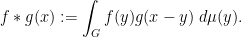
where  denotes the convolution operation
A variant of this result (expressed in the language of ergodic theory) appears in this paper of Bergelson, Host, and Kra; a combinatorial version of the Bergelson-Host-Kra result that is closer to Theorem 3 subsequently appeared in this paper of Ben Green and myself, but this theorem arguably appears implicitly in a much older paper of Bourgain. To see why Theorem 3 implies Theorem 1, we apply the theorem with  and
and  equal to a small multiple of
  to conclude that there is a Bohr set with
  and
and  such that

But from (2) we have the pointwise bound  , and Theorem 1 follows.
Below the fold, we give a short proof of Theorem 3, using an “energy pigeonholing” argument that essentially dates back to the 1986 paper of Bourgain mentioned previously (not to be confused with a later 1999 paper of Bourgain on Roth’s theorem that was highly influential, for instance in emphasising the importance of Bohr sets). The idea is to use the pigeonhole principle to choose the Bohr set to capture all the “large Fourier coefficients” of  , but such that a certain “dilate” of does not capture much more Fourier energy of than itself. The bound (3) may then be obtained through elementary Fourier analysis, without much need to explicitly compute things like the Fourier transform of an indicator function of a Bohr set. (However, the bound obtained by this argument is going to be quite poor – of tower-exponential type.) To do this we perform a structural decomposition of into “structured”, “small”, and “highly pseudorandom” components, as is common in the subject (e.g. in this previous blog post), but even though we crucially need to retain non-negativity of one of the components in this decomposition, we can avoid recourse to conditional expectation with respect to a partition (or “factor”) of the space, using instead convolution with one of the considered above to achieve a similar effect.
— 1. Proof of theorem —
Fix  . Let
. Let  be a large integer (depending only on ) to be chosen later. We will need a sequence

of small parameters, with each  assumed to be sufficiently small depending on all previous
  and on . (One should think of the as shrinking to zero incredibly fast, e.g.
  and
and  for
for  .)
.)
We then define an increasing sequence

of finite sets  of frequencies, as follows.
An easy induction using Plancherel’s theorem and (2) repeatedly gives the bounds

and

for all  .
.
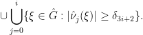
From Plancherel’s theorem we also have

As the are increasing, we thus see from the pigeonhole principle (if is sufficiently large depending on ) that there exists  such that

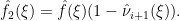
We now decompose

where


One can think of  as the “low frequency” (or “structured”, or “quasiperiodic”), “medium frequency” (or “small”), and “high frequency” (or “highly pseudorandom”) components of , where the notion of what it means for a frequency to be high or low is not determined by some preconceived notion of magnitude, but is instead adapted to the function itself. We will think of
  as the “main” term, and
  as “errors”.
Since is bounded in magnitude by  , and
, and  are non-negative with total mass , we have the
  bounds

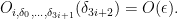
Now we give further bounds on  . We begin with
  :
:
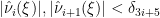
Lemma 4 ( has very small Fourier coefficients) We have

Proof: Let  . From the definition of and elementary Fourier analysis we have
If  , then from (5) we have

and the claim follows (since  has total mass one). Now suppose instead that
  . Then from (4) we have

for all  in the support of , and thus

and the claim again follows.
Now we control  :
:
Lemma 5 ( small in  ) We have

Proof: From the definition of and elementary Fourier analysis we have

We wish to bound this by  . From (7) we see that the contribution of those
  in
in  are acceptable. Now let us look at the contribution with
  . From (5) we have
for such , so this contribution to (9) is certainly acceptable thanks to (6). Now suppose that  . The argument in the proof of Lemma 4 shows that
  and
and  , and so this contribution is again acceptable thanks to (6).
Finally, we record the key properties of :
Lemma 6 ( continuous) is non-negative, has mean 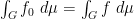 , and obeys the bound

whenever  and
and  .
.
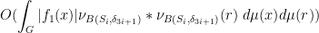
Proof: The first two properties are obvious, so we turn to the third. Since  and is bounded, it suffices to show that
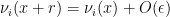
whenever and . But from (1) and the triangle inequality we have

for such  , and the claim follows from (2).
Now we can prove Theorem 3 with  . Splitting
  as above, we can decompose the left-hand side of (3) into
  terms, each of the form

for some 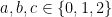 .
.
Let us consider a term for which  . We can bound this term by
which is  thanks to Lemma 5. Similar arguments hold for terms with
  or
or  , after shifting by
  or .
or .
Now let us consider a term for which  , that is to say

A short Fourier-analytic calculation reveals that this integral may be written as a sum
From (2) we have
and thus by Plancherel
Similarly, from (6) we have
and

and hence by Cauchy-Schwarz and the -torsion-free nature of , one has
for all . Combining these estimates with Lemma 4, we conclude that this contribution to (3) is
Similar arguments dispose of the terms for which  or
or  .
.
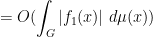
The only remaining term is when  , that is to say

From several applications of Lemma 6 we see that

for  in the support of this integrand. Thus this term may be written as

which on evaluating the integral simplifies to

but by the non-negativity of and Hölder’s inequality, this is at least

and the claim follows.

.
, introduce the function
to be the set
, increment
to
and return to step (ii).


11 comments
Comments feed for this article
28 April, 2014 at 12:45 am
mpetrache
Hello! I would like to ask a question: what fails to work for the estimates if one tries to get a result on lenght n>3 arithmetic progressions similar to this version of Roth-Kintchin theorem?
Also (probably this is a bit irrelevant) I guess in (5) there should be some “j” in the last term, right?
Thank you!
28 April, 2014 at 7:52 am
Terence Tao
Thanks for the correction!
With patterns of complexity greater than 1 (such as arithmetic progressions of length four and greater), what happens is that the Fourier pseudorandomness in Lemma 4 is no longer strong enough to control the contribution of (this is discussed extensively in Gowers’ paper on Szemeredi’s theorem for length four progressions). For k=4, it is possible to salvage this argument, but with all appearances of linear Fourier analysis arguments replaced by their quadratic Fourier analysis counterparts; this is done in my paper with Ben on the arithmetic regularity lemma that was linked to above. However, just as the k=3 argument relied on an analytic inequality, namely Holder’s inequality
  , the k=4 argument relies on an analytic inequality (roughly speaking, that
  when
when  takes values in a compact abelian group with Haar probability measure) which does not have an analogue for k=5 and higher, and the Khintchine type theorem is in fact false in that case, as was essentially demonstrated by Ruzsa in an appendix to the paper of Bergelson, Host, and Kra linked to above. (Of course, Szemeredi’s theorem for k>=5 can be established by other means.)
28 April, 2014 at 6:31 pm
Anonymous
I think the displayed equation (9) looks a little funny…
[Corrected, thanks – T.]
29 April, 2014 at 6:16 am
Anonymous
Is there a reason why $f_0,f_1,f_2$ are defined using double convolutions?
29 April, 2014 at 7:41 am
Terence Tao
The double comvolution obeys good
  bounds on the Fourier transform (i.e. Wiener algebra bounds), while
  only obeys good
  bounds on the Fourier transform. For the Fourier-analytic treatment of the
  terms,
  control of the Fourier transform becomes essential.
29 April, 2014 at 8:25 am
Anonymous
I was curious about using the double convolution in the definition of the functions $f_0,f_1,f_2$.
It seems to me that $f_0$ is still sufficiently smooth with a single convolution, $f_1$ still has small $L^2$ norm, and $f_2$ still has small Fourier coefficients.
29 April, 2014 at 8:45 am
Terence Tao
Hmm, you’re right, the double convolution is not needed here, even though it is needed to constrain the shift. I’ve edited the text appropriately to reflect this simplification to the argument.
10 March, 2016 at 11:22 am
Anonymous
Hi Professor Tao, I have trouble seeing how, in the proof of Lemma 2, the sets forming an open cover of G are translates of B(S,𝜌). Am I missing something?
10 March, 2016 at 11:32 am
Terence Tao
They are each contained in translates of (more specifically, they are contained in
  for any element
  of that set), but are not necessarily equal to such translates.
10 March, 2016 at 11:48 am
Anonymous
Pardon me for my sloppy question — I actually meant “contained in translates of $$ B(S,\rho) $$”. This I had trouble seeing, unless I assumed that each $$ \theta $$ used for the translation was of the form $$ (\xi \cdot y)_{\xi \in S} $$ for some $$ y \in G $$.
10 March, 2016 at 12:32 pm
Terence Tao
Let be a set of the form
  . If
. If  is empty then we are done, so suppose
  contains an element
  . Then for any other
  ,
,  , which implies that
  , so
, so  lies in the translate
  of
of  ,
,