Word maps close to the identity

While talking mathematics with a postdoc here at UCLA (March Boedihardjo) we came across the following matrix problem which we managed to solve, but the proof was cute and the process of discovering it was fun, so I thought I would present the problem here as a puzzle without revealing the solution for now.

The problem involves word maps on a matrix group, which for sake of discussion we will take to be the special orthogonal group of real matrices (one of the smallest matrix groups that contains a copy of the free group, which incidentally is the key observation powering the Banach-Tarski paradox).  Given any abstract word of two generators and their inverses (i.e., an element of the free group ), one can define the word map simply by substituting a pair of matrices in into these generators.  For instance, if one has the word , then the corresponding word map is given by

for .  Because contains a copy of the free group, we see the word map is non-trivial (not equal to the identity) if and only if the word itself is nontrivial.

Anyway, here is the problem:

Problem. Does there exist a sequence of non-trivial word maps that converge uniformly to the identity map?

To put it another way, given any , does there exist a non-trivial word such that for all , where denotes (say) the operator norm, and denotes the identity matrix in ?

As I said, I don’t want to spoil the fun of working out this problem, so I will leave it as a challenge. Readers are welcome to share their thoughts, partial solutions, or full solutions in the comments below.

Matrix identities as derivatives of determinant identities

The determinant of a square matrix obeys a large number of important identities, the most basic of which is the multiplicativity property

whenever are square matrices of the same dimension. This identity then generates many other important identities. For instance, if is an matrix and is an matrix, then by applying the previous identity to equate the determinants of and (where we will adopt the convention that denotes an identity matrix of whatever dimension is needed to make sense of the expressions being computed, and similarly for ) we obtain the Weinstein-Aronszajn determinant identity

This identity, which converts an determinant into an determinant, is very useful in random matrix theory (a point emphasised in particular by Deift), particularly in regimes in which is much smaller than .

Another identity generated from (1) arises when trying to compute the determinant of a block matrix

where is an matrix, is an matrix, is an matrix, and is an matrix. If is invertible, then we can manipulate this matrix via block Gaussian elimination as

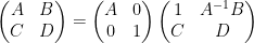
and on taking determinants using (1) we obtain the Schur determinant identity

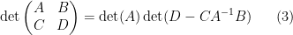
relating the determinant of a block-diagonal matrix with the determinant of the Schur complement of the upper left block . This identity can be viewed as the correct way to generalise the determinant formula

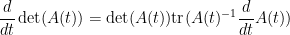
It is also possible to use determinant identities to deduce other matrix identities that do not involve the determinant, by the technique of matrix differentiation (or equivalently, matrix linearisation). The key observation is that near the identity, the determinant behaves like the trace, or more precisely one has

for any bounded square matrix and infinitesimal . (If one is uncomfortable with infinitesimals, one can interpret this sort of identity as an asymptotic as .) Combining this with (1) we see that for square matrices of the same dimension with invertible and invertible, one has

for infinitesimal . To put it another way, if is a square matrix that depends in a differentiable fashion on a real parameter , then we have the Jacobi formula

whenever is invertible. (Note that if one combines this identity with cofactor expansion, one recovers Cramer’s rule.)

Let us see some examples of this differentiation method. If we take the Weinstein-Aronszajn identity (2) and multiply one of the rectangular matrices by an infinitesimal , we obtain

applying (4) and extracting the linear term in (or equivalently, differentiating at and then setting ) we conclude the cyclic property of trace:

To manipulate derivatives and inverses, we begin with the Neumann series approximation

for bounded square and infinitesimal , which then leads to the more general approximation

for square matrices of the same dimension with bounded. To put it another way, we have

whenever depends in a differentiable manner on and is invertible.

We can then differentiate (or linearise) the Schur identity (3) in a number of ways. For instance, if we replace the lower block by for some test matrix , then by (4), the left-hand side of (3) becomes (assuming the invertibility of the block matrix)

while the right-hand side becomes

extracting the linear term in , we conclude that

As was an arbitrary matrix, we conclude from duality that the lower right block of is given by the inverse of the Schur complement:

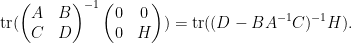
One can also compute the other components of this inverse in terms of the Schur complement by a similar method (although the formulae become more complicated). As a variant of this method, we can perturb the block matrix in (3) by an infinitesimal multiple of the identity matrix giving

By (4), the left-hand side is

From (5), we have

and so from (4) the right-hand side of (6) is

extracting the linear component in , we conclude the identity

which relates the trace of the inverse of a block matrix, with the trace of the inverse of one of its blocks. This particular identity turns out to be useful in random matrix theory; I hope to elaborate on this in a later post.

As a final example of this method, we can analyse low rank perturbations of a large () matrix , where is an matrix and is an matrix for some . (This type of situation is also common in random matrix theory, for instance it arose in this previous paper of mine on outliers to the circular law.) If is invertible, then from (1) and (2) one has the matrix determinant lemma

if one then perturbs by an infinitesimal matrix , we have

Extracting the linear component in as before, one soon arrives at

assuming that and are both invertible; as is arbitrary, we conclude (after using the cyclic property of trace) the Sherman-Morrison formula

for the inverse of a low rank perturbation of a matrix . While this identity can be easily verified by direct algebraic computation, it is somewhat difficult to discover this identity by such algebraic manipulation; thus we see that the “determinant first” approach to matrix identities can make it easier to find appropriate matrix identities (particularly those involving traces and/or inverses), even if the identities one is ultimately interested in do not involve determinants. (As differentiation typically makes an identity lengthier, but also more “linear” or “additive”, the determinant identity tends to be shorter (albeit more nonlinear and more multiplicative) than the differentiated identity, and can thus be slightly easier to derive.)

Exercise 1 Use the “determinant first” approach to derive the Woodbury matrix identity (also known as the binomial inverse theorem)

where is an matrix, is an matrix, is an matrix, and is an matrix, assuming that , and are all invertible.

Exercise 2 Let be invertible matrices. Establish the identity

and differentiate this in to deduce the identity

(assuming that all inverses exist) and thence

Rotating by then gives

which is useful for inverting a matrix that has been split into a self-adjoint component and a skew-adjoint component .

Pythagoras’ theorem

My colleague Ricardo Pérez-Marco showed me a very cute proof of Pythagoras’ theorem, which I thought I would share here; it’s not particularly earth-shattering, but it is perhaps the most intuitive proof of the theorem that I have seen yet.

In the above diagram, a, b, c are the lengths BC, CA, and AB of the right-angled triangle ACB, while x and y are the areas of the right-angled triangles CDB and ADC respectively. Thus the whole triangle ACB has area x+y.

Now observe that the right-angled triangles CDB, ADC, and ACB are all similar (because of all the common angles), and thus their areas are proportional to the square of their respective hypotenuses. In other words, (x,y,x+y) is proportional to . Pythagoras’ theorem follows.

Open question: What is a quantum honeycomb?

This problem lies in the highly interconnected interface between algebraic combinatorics (esp. the combinatorics of Young tableaux and related objects, including honeycombs and puzzles), algebraic geometry (particularly classical and quantum intersection theory and geometric invariant theory), linear algebra (additive and multiplicative, real and tropical), and the representation theory (classical, quantum, crystal, etc.) of classical groups. (Another open problem in this subject is to find a succinct and descriptive name for the field.) I myself haven’t actively worked in this area for several years, but I still find it a fascinating and beautiful subject. (With respect to the dichotomy between structure and randomness, this subject lies deep within the “structure” end of the spectrum.)

As mentioned above, the problems in this area can be approached from a variety of quite diverse perspectives, but here I will focus on the linear algebra perspective, which is perhaps the most accessible. About nine years ago, Allen Knutson and I introduced a combinatorial gadget, called a honeycomb, which among other things controlled the relationship between the eigenvalues of two arbitrary Hermitian matrices A, B, and the eigenvalues of their sum A+B; this was not the first such gadget that achieved this purpose, but it was a particularly convenient one for studying this problem, in particular it was used to resolve two conjectures in the subject, the saturation conjecture and the Horn conjecture. (These conjectures have since been proven by a variety of other methods.) There is a natural multiplicative version of these problems, which now relates the eigenvalues of two arbitrary unitary matrices U, V and the eigenvalues of their product UV; this led to the “quantum saturation” and “quantum Horn” conjectures, which were proven a couple years ago. However, the quantum analogue of a “honeycomb” remains a mystery; this is the main topic of the current post.