This week I am at the American Institute of Mathematics, as an organiser on a workshop on the universality phenomenon in random matrices. There have been a number of interesting discussions so far in this workshop. Percy Deift, in a lecture on universality for invariant ensembles, gave some applications of what he only half-jokingly termed “the most important identity in mathematics”, namely the formula

whenever  are
are  and
and  matrices respectively (or more generally,
  and
and  could be linear operators with sufficiently good spectral properties that make both sides equal). Note that the left-hand side is an
  determinant, while the right-hand side is a
  determinant; this formula is particularly useful when computing determinants of large matrices (or of operators), as one can often use it to transform such determinants into much smaller determinants. In particular, the asymptotic behaviour of determinants as
  can be converted via this formula to determinants of a fixed size (independent of
  ), which is often a more favourable situation to analyse. Unsurprisingly, this trick is particularly useful for understanding the asymptotic behaviour of determinantal processes.
There are many ways to prove the identity. One is to observe first that when are invertible square matrices of the same size, that  and
and  are conjugate to each other and thus clearly have the same determinant; a density argument then removes the invertibility hypothesis, and a padding-by-zeroes argument then extends the square case to the rectangular case. Another is to proceed via the spectral theorem, noting that
  and
and  have the same non-zero eigenvalues.
By rescaling, one obtains the variant identity

which essentially relates the characteristic polynomial of with that of . When  , a comparison of coefficients this already gives important basic identities such as
  and
and  ; when is not equal to
  , an inspection of the
  coefficient similarly gives the Cauchy-Binet formula (which, incidentally, is also useful when performing computations on determinantal processes).
Thanks to this formula (and with a crucial insight of Alice Guionnet), I was able to solve a problem (on outliers for the circular law) that I had in the back of my mind for a few months, and initially posed to me by Larry Abbott; I hope to talk more about this in a future post.
Today, though, I wish to talk about another piece of mathematics that emerged from an afternoon of free-form discussion that we managed to schedule within the AIM workshop. Specifically, we hammered out a heuristic model of the mesoscopic structure of the eigenvalues  of the Gaussian Unitary Ensemble (GUE), where is a large integer. As is well known, the probability density of these eigenvalues is given by the Ginebre distribution

where  is Lebesgue measure on the Weyl chamber
  ,
,  is a constant, and the Hamiltonian
  is given by the formula

At the macroscopic scale of  , the eigenvalues
  are distributed according to the Wigner semicircle law
Indeed, if one defines the classical location  of the
  eigenvalue to be the unique solution in
 ![{[-2\sqrt{n}, 2\sqrt{n}]}](https://s0.wp.com/latex.php?latex=%7B%5B-2%5Csqrt%7Bn%7D%2C+2%5Csqrt%7Bn%7D%5D%7D&bg=ffffff&fg=000000&s=0&c=20201002) to the equation
to the equation
then it is known that the random variable  is quite close to . Indeed, a result of Gustavsson shows that, in the bulk region when
  , is distributed asymptotically as a gaussian random variable with mean and variance
 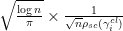 . Note that from the semicircular law, the factor
  is the mean eigenvalue spacing.
At the other extreme, at the microscopic scale of the mean eigenvalue spacing (which is comparable to  in the bulk, but can be as large as
  at the edge), the eigenvalues are asymptotically distributed with respect to a special determinantal point process, namely the Dyson sine process in the bulk (and the Airy process on the edge), as discussed in this previous post.
Here, I wish to discuss the mesoscopic structure of the eigenvalues, in which one involves scales that are intermediate between the microscopic scale and the macroscopic scale , for instance in correlating the eigenvalues and in the regime  for some
  . Here, there is a surprising phenomenon; there is quite a long-range correlation between such eigenvalues. The result of Gustavsson shows that both and behave asymptotically like gaussian random variables, but a further result from the same paper shows that the correlation between these two random variables is asymptotic to
  (in the bulk, at least); thus, for instance, adjacent eigenvalues
  and are almost perfectly correlated (which makes sense, as their spacing is much less than either of their standard deviations), but that even very distant eigenvalues, such as
  and
and  , have a correlation comparable to
  . One way to get a sense of this is to look at the trace

This is also the sum of the diagonal entries of a GUE matrix, and is thus normally distributed with a variance of . In contrast, each of the (in the bulk, at least) has a variance comparable to  . In order for these two facts to be consistent, the average correlation between pairs of eigenvalues then has to be of the order of .
Below the fold, I give a heuristic way to see this correlation, based on Taylor expansion of the convex Hamiltonian  around the minimum
  , which gives a conceptual probabilistic model for the mesoscopic structure of the GUE eigenvalues. While this heuristic is in no way rigorous, it does seem to explain many of the features currently known or conjectured about GUE, and looks likely to extend also to other models.
— 1. Fekete points —
It is easy to see that the Hamiltonian is convex in the Weyl chamber, and goes to infinity on the boundary of this chamber, so it must have a unique minimum, at a set of points  known as the Fekete points. At the minimum, we have
  , which expands to become the set of conditions
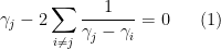
for all  . To solve these conditions, we introduce the monic degree polynomial
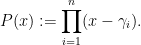
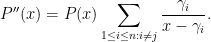
Differentiating this polynomial, we observe that

and

Using the identity

followed by (1), we can rearrange this as
Comparing this with (2), we conclude that

or in other words that  is the
  Hermite polyomial

Thus the Fekete points  are nothing more than the zeroes of the Hermite polynomial.
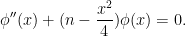
Heuristically, one can study these zeroes by looking at the function

which solves the eigenfunction equation
Comparing this equation with the harmonic oscillator equation 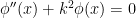 , which has plane wave solutions
 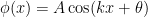 for
for  positive and exponentially decaying solutions for negative, we are led (heuristically, at least) to conclude that
  is concentrated in the region where
  is positive (i.e. inside the interval
 ![{[-2\sqrt{n},2\sqrt{n}]}](https://s0.wp.com/latex.php?latex=%7B%5B-2%5Csqrt%7Bn%7D%2C2%5Csqrt%7Bn%7D%5D%7D&bg=ffffff&fg=000000&s=0&c=20201002) ) and will oscillate at frequency roughly
) and will oscillate at frequency roughly  inside this region. As such, we expect the Fekete points to obey the same spacing law as the classical locations
  ; indeed it is possible to show that
 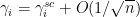 in the bulk (with some standard modifications at the edge). In particular, we have the heuristic

for  in the bulk.
Remark 1 If one works with the circular unitary ensemble (CUE) instead of the GUE, the Fekete points become equally spaced around the unit circle, so that this heuristic essentially becomes exact.
— 2. Taylor expansion —
Now we expand around the Fekete points by making the ansatz

thus Gustavsson’s result predicts that each  is normally distributed with standard deviation
  (in the bulk). We Taylor expand

We heuristically drop the cubic and higher order terms. The constant term  can be absorbed into the partition constant , while the linear term vanishes by the property
  of the Fekete points. We are thus lead to a quadratic (i.e. gaussian) model
for the probability distribution of the shifts , where  is the appropriate normalisation constant.
Direct computation allows us to expand the quadratic form  as
as

The Taylor expansion is not particularly accurate when  and
and  are too close, say
  , but we will ignore this issue as it should only affect the microscopic behaviour rather than the mesoscopic behaviour. This models the as (coupled) gaussian random variables whose covariance matrix can in principle be explicitly computed by inverting the matrix of the quadratic form. Instead of doing this precisely, we shall instead work heuristically (and somewhat inaccurately) by re-expressing the quadratic form in the Haar basis. For simplicity, let us assume that is a power of
  . Then the Haar basis consists of the basis vector

together with the basis vectors

for every discrete dyadic interval  of length between and , where
  and
and  are the left and right halves of
  , and
, and  ,
,  are the vectors that are one on
  respectively and zero elsewhere. These form an orthonormal basis of
  , thus we can write

for some coefficients  .
.
From orthonormality we have

and we have

where the matrix coefficients  are given by
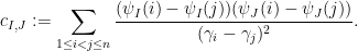
A standard heuristic wavelet computation using (3) suggests that is small unless and  are actually equal, in which case one has

(in the bulk, at least). Actually, the decay of the away from the diagonal  is not so large, because the Haar wavelets
  have poor moment and regularity properties. But one could in principle use much smoother and much more balanced wavelets, in which case the decay should be much faster.
This suggests that the GUE distribution could be modeled by the distribution
for some absolute constant  ; thus we may model
  and
and  for some iid gaussians
  independent of
  . We then have as a model

for the fluctuations of the eigenvalues (in the bulk, at least), leading of course to the model
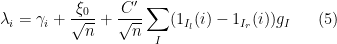
for the fluctuations themselves. This model does not capture the microscopic behaviour of the eigenvalues such as the sine kernel (indeed, as noted before, the contribution of the very short (which corresponds to very small values of  ) is inaccurate), but appears to be a good model to describe the mesoscopic behaviour. For instance, observe that for each there are
  independent normalised gaussians in the above sum, and so this model is consistent with the result of Gustavsson that each is gaussian with standard deviation
  . Also, if , then the expansions (5) of
  share about
  of the
  terms in the sum in common, which is consistent with the further result of Gustavsson that the correlation between such eigenvalues is comparable to .
If one looks at the gap  using (5) (and replacing the Haar cutoff
  by something smoother for the purposes of computing the gap), one is led to a heuristic of the form

The dominant terms here are the first term and the contribution of the very short intervals . At present, this model cannot be accurate, because it predicts that the gap can sometimes be negative; the contribution of the very short intervals must instead be replaced some other model that gives sine process behaviour, but we do not know of an easy way to set up a plausible such model.
On the other hand, the model suggests that the gaps are largely decoupled from each other, and have gaussian tails. Standard heuristics then suggest that of the  gaps in the bulk, the largest one should be comparable to
  , which was indeed established recently by Ben Arous and Bourgarde.
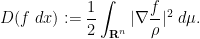
Given any probability measure  on (or on the Weyl chamber) with a smooth nonzero density, one can can create an associated heat flow on other smooth probability measures
  by performing gradient flow with respect to the Dirichlet form
Using the ansatz (4), this flow decouples into a system of independent Ornstein-Uhlenbeck processes
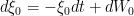
and
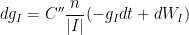
where  are independent Wiener processes (i.e. Brownian motion). This is a toy model for the Dyson Brownian motion. In this model, we see that the mixing time for each
  is
is  ; thus, the large-scale variables ( for large ) evolve very slowly by Dyson Brownian motion, taking as long as
  to reach equilibrium, while the fine scale modes ( for small ) can achieve equilibrium in as brief a time as
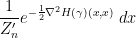
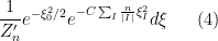
  , with the intermediate modes taking an intermediate amount of time to reach equilibrium. It is precisely this picture that underlies the Erdos-Schlein-Yau approach to universality for Wigner matrices via the local equilibrium flow, in which the measure (4) is given an additional (artificial) weight, roughly of the shape
  , in order to make equilibrium achieved globally in just time
  , leading to a local log-Sobolev type inequality that ensures convergence of the local statistics once one controls a Dirichlet form connected to the local equilibrium measure; and then one can use the localisation of eigenvalues provided by a local semicircle law to control that Dirichlet form in turn for measures that have undergone Dyson Brownian motion.


11 comments
Comments feed for this article
18 December, 2010 at 4:10 pm
Anonymous
Shouldn’t the identity matrix be “I” instead of “1”?
[Either notation is appropriate. In the modern abstract algebra, the multiplicative identity of any ring is often denoted 1, for much the same reason that the additive identity is often denoted 0. -T]
19 December, 2010 at 7:01 am
Marek
The equation for the harmonic oscillator is missing a sign.
[Corrected, thanks -T]
22 December, 2010 at 1:23 pm
Anonymous
Is there a website for this workshop
23 December, 2010 at 11:58 pm
Ben Golub
“namely the Dyson sine process in the bulk (and the Airy process on the edge), as discussed in this previous post” is missing a link
[Corrected, thanks – T.]
24 December, 2010 at 12:52 am
Ben Golub
Sorry for posting twice, but there is one more possible typo and a question
On the line following
“From orthonormality we have”, it seems the upper bound of the summation should be n.
after “A standard heuristic wavelet computation”: it seems that naively plugging in $I=J$ in the summation defining $c_{I,J}$ makes the expression $(\psi_I – \psi_J)^2$ equal to $0$ (interpreting squaring as taking the dot product of the vector with itself). It seems I am missing something simple — any help would be appreciated.
[Corrected, thanks – T.]
14 January, 2011 at 7:14 am
The 3rd lecture in 2011 Spring « Y.-K. Lau's Weblog
[…] was drawn attention to (1) by an article in Tao’s blog. A proof (different from ours) is given there. Professor Terence Tao is a […]
3 February, 2011 at 2:44 pm
Subsynchronous Resonance in Power Systems | BUKU PDF
[…] The mesoscopic structure of GUE eigenvalues (terrytao.wordpress.com) […]
23 February, 2011 at 6:54 am
Topics in random matrix theory « What’s new
[…] which was based primarily on my graduate course in the topic, though it also contains material from some additional posts related to random matrices on the blog. It is available online here. As usual, […]
8 June, 2011 at 10:52 am
Djalil
It seems that the det(1+AB)=det(1+BA) identity is attributed to Sylvester: http://en.wikipedia.org/wiki/Sylvester%27s_determinant_theorem
13 January, 2013 at 12:36 pm
Matrix identities as derivatives of determinant identities « What’s new
[…] which relates an determinant with an determinant, is very useful in random matrix theory (a point emphasised in particular by Deift), particularly in regimes in which is much smaller than […]
20 November, 2016 at 11:55 pm
Miklós Kornyik
After inroducing the orthonormal Haar basis you write that sum_j x_j^2/2 = sum_k xi_k^2. Where does the 1/2 come from? Shouldn’t it be just sum_j x_j^2 = sum_k xi_k^2 ?
[Corrected, thanks – T.]