[This post is authored by Emmanuel Kowalski.]
This post may be seen as complementary to the post “The parity problem in sieve theory“. In addition to a survey of another important sieve technique, it might be interesting as a discussion of some of the foundational issues which were discussed in the comments to that post.
Many readers will certainly have heard already of one form or another of the “large sieve inequality”. The name itself is misleading however, and what is meant by this may be something having very little, if anything, to do with sieves. What I will discuss are genuine sieve situations.
The framework I will describe is explained in the preprint arXiv:math.NT/0610021, and in a forthcoming Cambridge Tract. I started looking at this first to have a common setting for the usual large sieve and a “sieve for Frobenius” I had devised earlier to study some arithmetic properties of families of zeta functions over finite fields. Another version of such a sieve was described by Zywina (“The large sieve and Galois representations”, preprint), and his approach was quite helpful in suggesting more general settings than I had considered at first. The latest generalizations more or less took life naturally when looking at new applications, such as discrete groups.
Unfortunately (maybe), there will be quite a bit of notation involved; hopefully, the illustrations related to the classical case of sieving integers to obtain the primes (or other subsets of integers with special multiplicative features) will clarify the general case, and the “new” examples will motivate readers to find yet more interesting applications of sieves.
— Setting up the sieve —
The objects to sieve will be in a fixed set  , typically infinite. The “sieve” is related to the assumed existence of a set of surjective maps
  , where
  runs through another (arbitrary) set
  , and
, and  is a finite set. Combinatorialists can think of these maps as a family of colorings of , and number-theorists can think of “reduction” maps modulo , in the case where is a subset of prime numbers. Indeed, the classical case occurs with
  , the set of primes, and
  being the reduction map.
We now want to define sifted sets and try to “count” them. This is where classically one would look at a discrete interval of integers, and one could think of taking a finite subset of as a generalization. However, we will generalize this by looking at an arbitrary measure space  , such that
  is finite, and assume there is a map (measurable in an obvious sense)
  from
from  to , and instead of “counting”, we will try to understand the measure (under
  ) of sifted sets, of the following type:

whenever subsets  have been chosen, say for a finite subset
  of .
of .
Classically, we have  for some integer
  , is the counting measure, and one might consider
  , for prime, to be e.g.,
  modulo : if is the set of primes
  , we see that
  is (essentially) the set of twin primes between
  and . It is clear from this that in most applications we will really have a sequence of sets (with attending and
  ), depending on some parameter (here ), and it will be when this parameter gets large that the results will be interesting. In particular, we need to be careful about the uniformity of our results if they are going to be useful.
— First examples —
There are a great many different settings that can be phrased in such a way. Here are a few, beyond the case of integers, which are related to existing results and can be described fairly easily:
Example 1. If we have a probability space  , and a (finite) family of events
  ,
,  , we can set up a sieve by taking
  ,
,  ,
,  ,
,  , and letting
  be the characteristic function of
  . Then the sifted set
  is simply the event which is the intersection of the complements of , if we take
  ; the probability of can be expressed using the usual inclusion-exclusion formula.
Example 2. Gallagher used the large sieve in several variables to study the typical Galois group of a monic integral polynomial with height  ,
,  getting large. Here can be defined to be the space of monic integral polynomials of degree
  , the subset of those with height
  , is the set of primes, the space of monic polynomials of degree over the finite field
  , and is the obvious restriction map.
Example 3. Serre used a variant of the large sieve to study the density of quadratic forms over  in
in  variables which have a non-trivial rational zero. Here, can be described as the set of coefficients describing the quadratic forms, the sets are those quadratic forms with height
  , with getting large, is the set of primes, and is the reduction modulo
  .
.
Example 4. Poonen used a very nice sieve to find the density, among homogeneous polynomials ![f\in \mathbf{F}_q[x_0,...,x_n]](https://s0.wp.com/latex.php?latex=f%5Cin+%5Cmathbf%7BF%7D_q%5Bx_0%2C...%2Cx_n%5D&bg=ffffff&fg=545454&s=0&c=20201002) , with coefficients in a finite field
, with coefficients in a finite field  , of those such that the intersection
  is smooth, where
  is a fixed smooth subvariety
  of projective -space. One can set up the sieve more or less as follows: is the set of all homogeneous polynomials with coefficients in , for
  fixed, is the subset of polynomials of degree (and the normalized counting measure on ), is the set of closed points of (which can be thought-of simply as the set of Galois-orbits of points of over an algebraic closure of ) and
  , for
, for  such a point, maps to the -vector space of possible Taylor expansions of order 1. Poonen uses as sieving sets the
  which characterize to be a singular point, so that an
  survives sieving by all precisely when is smooth.
We will give a few more recent examples later in this post.
— Heuristics —
Now, we will describe the general large-sieve inequality which can be used in many cases to obtain an upper bound for the measure of the sifted set. Let us try first to guess what the “right” answer should be, which will highlight the need for a further piece of data, which is usually merely implicit in the classical cases.
The heuristic value for the measure of the sifted set arises from two fairly natural assumptions: first, one might expect that the various should be “independent”, so the measure of the sifted set should be roughly equal to
 (1)
(1)
where  is the (normalized) image measure on of via
  obtained by composition:

This measure depends on (hence on some unspecified asymptotic parameter, such as the length of the interval of integers considered) and may be hard to understand; however, the second natural assumption is that this measure should be close to some “natural” measure  on which is independent of (if has some natural measure, it could be the image of this measure under ). In other words, we may hope that
  , for
, for  , becomes equidistributed with respect to such a measure.
In the classical case, integers in large intervals are uniformly distributed modulo any fixed prime, so  in this case. Note that assuming some form of asymptotic equidistribution is typically the content of standard “sieve axioms”, introducing sieve remainder terms measuring the default of exact equidistribution. In all the examples above, the target set are finite abelian groups, and the natural probability density is also the normalized counting measure, except in the case of inclusion-exclusion; there the natural measure is the distribution law of the characteristic function of : it maps
  ,
,  .
.
— Further examples —
Here are now the promised “new” examples, which in particular show further examples of non-trivial sieve settings, and less trivial measures on the finite sets .
Example 5. Let  be an elliptic curve defined over the rationals, given in Weierstrass form
  with
with  ,
,  integers. We can take
  , the finitely generated Mordell-Weil group of rational points on
  , the set of primes (not dividing the discriminant for simplicity),
  the image of under the reduction map modulo
  . In general, this image is badly understood (it certainly is not equal to the group of points on the reduction of modulo , in most cases, for instance because the latter grows with , whereas may well be finite). If we take
  to be the origin of the group law, the sifted set has an interesting interpretation: it is the set of -integer solutions of the equation which “is” , where is the set of primes dividing the discriminant (i.e., it is the set of solutions to the equation where the denominators of and
  are divisible only by those primes). In particular, in contrast with classical sieves, those points are examples of interesting elements which survive after “infinite” sieving (though a famous theorem of Siegel states there are only finitely many).
Example 6. Let  , and a fixed finite symmetric set of generators (e.g., is the set of elementary matrices with
  off the diagonal). For a prime , let
  be reduction modulo ; it is not obvious, but true, that the image is
  for all primes . The natural measure is again the counting measure on . We can define different types of sets to sieve (balls in word length or archimedean metric for instance), but one that has interest as being quite different-looking from the standard ones is the following: take to be an abstract probability space, and
  a
a  -valued random variable
  obtained as the
  -th step of a random walk defined by
  ,
,  , where the steps
  are independent, uniformly distributed -valued random variables (with
  for all
  ); for instance, may be chosen independently and uniformly at random in . In this setting, interesting sifted sets might be those where
  is a matrix with prime or almost prime entries (in this case the setup is closely related to ongoing work of Bourgain, Gamburd, and Sarnak, and other collaborators such as J. Liu, A. Nevo), or those has for instance a reducible characteristic polynomial, or one with small splitting field. This type of setting was considered first by I. Rivin, with fairly remarkable applications in low-dimensional topology and for the theory of free-group automorphisms. One can do this type of things also for other discrete groups, of course.
Example 7. The last example is studied by Zywina in his preprint “The large sieve and Galois representations”, and is a number field analogue of the sieve for Frobenius over function fields considered earlier by myself (the latter is notationally a bit more complicated). We select a special case again for concreteness, and disregard for simplicity some issues of ramification. Let be an elliptic curve without complex multiplication. We consider for the set of conjugacy classes in the group which is the image of the Galois group of under the natural action on all torsion points of ; by work of Serre, it is known that is naturally isomorphic to an open subgroup of  . We take to be the set of primes such that
  , the Galois group of the action on -torsion points, is isomorphic to
  : the result of Serre mentioned above implies that contains all primes except finitely many.There is a surjection
  , and correspondingly a surjective map where is the set of conjugacy classes in . On , the natural measure maps a conjugacy class
  to
to  ; since is not abelian, this is not counting measure on . Now we take to be the set of prime numbers
  , for some , which do not divide the discriminant of . The map from to maps to the conjugacy class of the Frobenius automorphism at (it is here that some care with ramification is needed to be precise).
Note that the equidistribution statement for a fixed is valid, and is a special case of the Chebotarev Density Theorem: for any conjugacy class in , we have 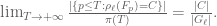
What are the applications of such a sieve setting? They arise because  has the following properties: the trace of
  (seen as an element of ) is the residue class modulo of the integer
  such that

In particular, controlling the conjugacy class of implies that the order of the curve modulo is (somehow) controlled, and these orders (or equivalently) control (at least conjecturally!) much of the arithmetic properties of the elliptic curve. In particular, recall that the Birch and Swinnerton-Dyer conjecture states that the rank of  should be the order at
  of the Euler product

Certainly, one can see how sieving in this context will lead to information on, say, almost-prime values of  , and many other arithmetic properties of the which are of great importance for instance in understanding some algorithms such as elliptic curve primality proving, elliptic curve cryptography, etc.
— Two sieve inequalities —
Coming back to the “large sieve inequalities”, we mentioned that they will provide one possible way to get upper bounds for the measure of , which are often comparable in size with the “expected” measure (1) above. There are two forms, which are inspired by the corresponding inequalities for integers due to Renyi and Montgomery respectively. Both depend on bounding a further quantity  , which is the crucial ingredient, and which is explained below (without knowing something about , the inequalities are useless; they should be read assuming that is close to , possibly up to a constant multiplicative factor).
I. Renyi’s sieve takes the form

where  is the number of
  such that
  , while
  is the “expected” value of this quantity, namely the sum over of
  .
.
So there is a clear interpretation: if is indeed close to , this means that is close to for “most” (in mean-square sense). In the case of counting primes, this inequality becomes the Turán inequality

which is known to be sharp (in fact there is an asymptotic formula of this size for the left-hand side).
In the case of Example 5 (elliptic curves), this gives some lower bound for the number of prime divisors of the denominator of “most” rational points (not without some extra work; and note that the proof require the use of Siegel’s Theorem: it does not provide another approach to it).
In general, note that we obtain the bound

for the measure of the sifted set, using positivity. This is weak; in the case of primes, when  tends to zero (it gives the bound
  for the number of primes
  ), but quite strong when is fairly large (bounded below); indeed, these are the situations which characterize what Linnik called the “large” sieve.
II. The second sieve inequality is stronger in case the local densities are small, in fact as strong qualitatively as the best “small” sieves. (But of course small sieve theory is developed a lot looking at lower bounds, which the large sieve does not approach directly — see the former post on the parity problem).
Here the idea is to combine the to look at the possible “multi-colorings”  , which classically means looking at the reductions modulo square-free integers, not only modulo primes.
Abstractly, this is done as follows: let  , for
, for  a finite subset of , be the product of for
  . Define
  in the obvious manner, but notice it may not be surjective. If it is, this means some analogue of the Chinese Remainder Theorem holds, and this may be very difficult to show (think about the case of elliptic curves). Similarly, having chosen , we can define
  as the product over elements of . Now choose an arbitrary finite set
  of finite subsets of ; e.g., could correspond by unique factorization to the set of all square-free integers
  , if is the set of primes at most
  .
.
We now have

where is as above, and will be explained below, and

Now this may look strange, but observe the following: if is the set of all subsets of , a moment’s thought reveals that
i.e., for  , the right-hand side of the large-sieve inequality is exactly the expected value in (1). The problem is that, typically, would be too large if is that big (this is shown for instance by the problem of explosion of the remainder term in applying the Eratosthenes-Legendre sieve to compute the number of primes less than ). The interpretation of this is then similar to that of the earlier sieves by V. Brun: using all subsets of (all integers divisible by primes
  ) is too costly, but a suitable “cutoff” yields approximations to the truth which can remain very useful. (One case where one can take so large is for Example 1, if the event are independent so that by the very definition of independence, the probability of the sifted set is exactly

and it turns out that in this case one has exactly  , so that
the large-sieve inequality is sharp in the full generality considered).
Now we need finally to define . The reason it was delayed is
that it will need yet more notation…
First, for each in , let  be the finite dimensional Hilbert space of functions of mean-zero on , i.e., of those such that

(with the inner product defined using the density ).
Select (arbitrarily) an orthonormal basis  of . Then consider the set
  of functions on of the type

where  is an element of the chosen basis of . Those functions form themselves an orthonormal basis for a “primitive” subspace of the space of functions on , with respect to the “product” inner-product on .
Finally, is defined to be the least non-negative real number such that the inequality

holds for any square-integrable function  on . For Renyi’s inequality, is simply the set of singletons
  for .
for .
One can see quite easily that is independent of the choice of basis (but practical estimates may well depend on a clever selection) by interpreting it as the norm of some operator between Hilbert spaces.
Let’s look at the classical example of integers: there, is the space of functions on which sum to zero, and a particular basis is given by the additive characters
for all non-zero  . Extending to all $m$, by the Chinese Remainder Theorem, amounts to looking at characters

of  with
with  coprime with . So the defining inequality for sieving
  using square-free numbers up to is

It is classical, by now, that  . The first bound of this strength being due to Bombieri, though this particular value is due to Montgomery-Vaughan and Selberg independently. In fact, stronger analytic inequalities are known, there it is not necessary to restrict to square-free on the left-hand side, and in fact one can look at arbitrary sets of well-spaced points in
  . This classical theory is very-well described in Montgomery’s survey paper. [Incidentally, reading this paper was the subject of my first-year project at E.N.S. Lyon under the direction of É. Fouvry and H. Daboussi, and it is quite remarkable how much of my mathematical work has involved the large-sieve in one way or another…]
— An approach to concrete sieve estimates —
Here is the most standard way to estimate directly . It relies on duality: the defining inequality is equivalent with

for arbitrary complex numbers  . Expanding the left-hand side, we find a quadratic form with coefficients

with  and
and  . Those correlation coefficients then must be estimated. One expects that

where the remainder R is estimated uniformly and explicitly, and is small compared with , at least if and are not “too big” (in the appropriate sense). Then we have

and this will have the desired feature of being close to if and are suitably chosen.
Here are the two most important new examples where this approach gives strong results, and leads to links with very deep principles of harmonic analysis and number theory.
In the setting of Example 6 (and its generalizations), i.e., sieve for discrete groups and random walks, a natural basis is given by the matrix coefficients of irreducible unitary representations of the finite groups  . Then estimating
  turns out to be very cleanly linked with Property
  for the congruence quotients of
  (or Property (T), though that applies only for at least
  ). Recall that this property states that there is a positive
  such that, for any
  , any map

where  is the unitary group of a finite-dimensional Hilbert space of dimension
  , either there is a vector
  invariant under all
  ,
,  , or for any unit vector
  , there exists
  (recall is a generating set of ) such that

In other words, if a vector is not invariant under all , it is uniformly non-invariant. This property is also equivalent with the fact that the Cayley graphs of the congruence quotients form a family of expanders.
(Note: we do not currently necessarily need fine knowledge of the character table of , as described at least partly through Deligne-Lusztig characters, though, when is large, this can lead to small improvements in estimates, and interesting problems).
In Example 7, since we work with conjugacy classes, the natural basis is the set of characters of irreducible unitary representations of . Estimating is then a problem of analytic number theory, amounting to uniform quantitative estimates for partial sums of coefficients (at primes) of Artin
-functions. As such, there exist unconditional, but fairly weak, results, and much stronger ones when assuming the Generalized Riemann Hypothesis.
When dealing with the function field analogue, the Riemann Hypothesis is known, due to the amazing work of Deligne [in my mind, the most important number-theory result of the 20th century], building on the foundations of Grothendieck. However, this only gives a (very strong) result for fixed  ,
,  , a priori; getting uniform bounds is not trivial, and because the remainder terms after applying the Grothendieck-Lefschetz trace formula and the Riemann Hypothesis involve the dimension of some étale cohomology groups depending on and , some uniform estimates for those so-called Betti numbers are required. They are proved either by analyzing the ramification behavior of the analogues of the Artin representations, or (for higher-dimensional parameter spaces) by adapting an induction method of Katz.
In applying concretely the sieve for Frobenius, it should be mentioned
that one of the main issues is in fact to compute precisely! This is a completely new phenomenon compared with the classical sieves, where is perfectly known and understood. Here, this amounts to computing certain Galois groups, such as those of torsion points on elliptic curves, or their analogues for function fields (which are often called monodromy groups because of their geometric origin). Serre’s theorem quoted above for non CM elliptic curves is one of the most famous examples, but the “baby” example of this is the fact that cyclotomic polynomials are irreducible over $\mathbf{Q}$ (since this means that the Galois groups of cyclotomic extensions, generated by roots of unity, are “as big as possible”, which is usually the desired outcome). In the first application of the sieve for Frobenius, which concerned a conjecture of Katz already considered by N. Chavdarov, I used an unpublished result of J-K. Yu which has recently been given a new proof by C. Hall.


6 comments
Comments feed for this article
9 August, 2007 at 6:15 am
Jordan Ellenberg
Emmanuel,
I’ve only just started reading this enjoyable post! But let me make a couple of comments off the bat.
1. In Poonen’s theorem (your example 4), the “sieve-style” method really only works for the points of small degree — there is a very clever trick involving Frobenius to deal with the points of large degree (section 2.3 of Poonen’s paper.) But maybe this is what you meant by “more or less” — or maybe to you this material in section 2.3 can be thought of as “sieve-style” as well, in which case I’d like to hear more about it!
2. Yu’s unpublished theorem was also reproved by Jeff Achter and Rachel Pries, independently of Hall.
9 August, 2007 at 11:06 am
Emmanuel Kowalski
Hello Jordan !
(1) This is absolutely correct; what I wanted to say was simply that
the framework of Poonen’s work, which is quite unusual by the usual
standards of classical analytic number theory, does fall within the
general framework I described (a good test that it is at least close to the
“right” one, although whether one can expect a perfect abstract theory for
something like this is not clear at all). In fact, in sieve-theoretic terms,
Poonen’s application is something like a “zero-dimensional sieve”, which
is quite far from the standard “large-sieve” (very few residue classes are excluded, instead of a positive proportion). This means in particular that
it is possible to expect an asymptotic formula with a positive density, though proving such a formula is of course quite difficult usually (see for instance the remarkable recent work of Helfgott proving that values of
a cubic polynomial evaluated at primes represent the right number of squarefree values, when there is no trivial obstruction). For a zero
dimensional sieve, the large sieve useless results in general.
(2) I know of this work of Achter and Pries, but actually I was thinking of
the stronger version of Yu’s theorem for one-parameter families
y^2=f(x)(x-t)
and as far as I understood their paper, this does not follow from their
approach (but I may be mistaken…)
15 August, 2007 at 9:57 am
Jesse Kass
A) It should be noted that (as I understand it) Yu’s proof of this monodromy result uses a technique that is entirely different from the technique used both in Hall’s paper and Achter-Pries’ paper. For the families considered by Achter and Pries, his proof is fundamentally topological and uses the description of the fundamental group of the parameter space as a briad group. He handles the case of an arbitrary base field by proving a comparison result.
B) Kowalski is correct that the Achter and Pries do not compute the monodromy for the family (considered as a family in the variable t). Furthermore, their technique can not be extended to handle this
family without some additional work.
Achter and Pries study the family
given by allowing to be any d-tuple of distint points. Their technique is to partially compactify the family by adding in curves of compact type (curves with compact Jacobian). The boundary looks like a product of spaces of the same type but of smaller dimension, so the monodromy group can be computed inductively. Achter and Pries then use a result about semi-continuity of mondromy under degeneration to compare the monodromy group of the boundary to the monodromy group of
  .
.
One way of extending this technique would be to put the into a larger family of smooth curves by allowing the coefficients of f(x) to vary in some continuous manner. One could try to do this in such a way so that the monodromy group of
  is the same as the monodromy group of the larger family. This larger family would then be a family for which it is natural to try to apply the technique from the Achter-Pries paper to.
The difficulty is that it is not immediately clear to me how to do this in such a manner that the larger family admits a partial compactification by curves of compact type. The wandering point (t,0) on the curve is the main source of difficulties.
For a partial compactification by curves that are not of compact type, it may still be possible to extend the method, but the difficulty lies proving an appropriate semi-continuity result. When all the curves in the family are of compact type, the monodromy group is the group associated to a sheaf (the sheaf ) that is locally constant on the entire partial compactification. This fact is used in a fundamental way by Achter and Pries and is no longer true when the family includes curves that are not of compact type.
16 August, 2007 at 2:01 am
Emmanuel Kowalski
Hello,
Thanks for the information on the methods of Achter and Pries, which are a bit far away from my current knowledge of algebraic geometry.
Incidentally there’s another question I’ve been wondering about concerning the families , which is whether the curves in the family are generically ordinary. (This is partly motivated by applications where both big monodromy and ordinarity are useful, e.g. this paper). I used to think this would probably be the case, but it’s not so clear since Achter and Pries have extended their results to get big monodromy results for the moduli spaces of curves with given
  -rank (arXiv:0707.2110), which implies in particular the existence of one-parameter families of curves with big monodromy, but not ordinary. (Though, of course, not necessarily of the form above.) (Katz had mentioned having found such families, but without details.)
16 August, 2007 at 8:29 am
Jesse Kass
Hello,
I think that the curves in the family y^2 = f(x) (x-t) are generically ordinary, at least for f(x) a general polynomial. I know that the generic hyperelliptic curve of genus g is ordinary and I think that the same kind of technique can be applied to your question.
Here is a sketch of the argument: Fix an integer d and consider the family
V_d:
y^2 = f(x)(x-t)
considered as a family over an open subset of A^{d-1} \times A^1 by varying both t and the coefficients of f(x) in a continuous manner. If this family is generically ordinary, then it follows that the family y^2 = g(x) (x-t) is generically ordinary for g(x) a general polynomial.
Now to prove that the larger family is generically ordinary, we induct on d. For d small (d <= 6), the family V_d contains every smooth curve of appropriate genus so we are ok.
For the inductive step, first compactify V_d by adding in nodal hyperelliptic curves. Now one can construct lots of ordinary curves that lie on the boundary of V_d by taking two curves in V_d’with d’ <d and gluing them together at a point. A deformation theory argument shows that these nodal, ordinary curves can be deformed into smooth, ordinary curves that lie in the interior of V_d. This proves that the generic element of V_d is ordinary.
Technical Note: For the inductive step, it is probably better to work with a finite quotient of V_d that has a nice moduli theoretic interpretation and then use a standard compactification of that space rather than to work with V_d directly.
20 November, 2008 at 1:13 pm
Marker lecture IV: sieving for almost primes and expanders « What’s new
[…] The selection of the sieve weights is now a well-developed science (see also my earlier post, and Kowalski’s guest post, on this topic), and Bourgain, Gamburd and Sarnak basically use off-the-shelf sieves (in […]