Today I’d like to discuss (part of) a cute and surprising theorem of Fritz John in the area of non-linear wave equations, and specifically for the equation
 (1)
(1)
where  is a scalar function of one time and three spatial dimensions.
The evolution of this type of non-linear wave equation can be viewed as a “race” between the dispersive tendency of the linear wave equation
 (2)
(2)
and the positive feedback tendencies of the nonlinear ODE
 . (3)
. (3)
More precisely, solutions to (2) tend to decay in time as  , as can be seen from the presence of the
  term in the explicit formula
![u(t,x) = \frac{1}{4\pi t} \int_{|y-x|=t} \partial_t u(0,y)\ dS(y) + \partial_t[\frac{1}{4\pi t} \int_{|y-x|=t} u(0,y)\ dS(y)],](https://s0.wp.com/latex.php?latex=u%28t%2Cx%29+%3D++%5Cfrac%7B1%7D%7B4%5Cpi+t%7D+%5Cint_%7B%7Cy-x%7C%3Dt%7D+%5Cpartial_t+u%280%2Cy%29%5C+dS%28y%29+%2B+%5Cpartial_t%5B%5Cfrac%7B1%7D%7B4%5Cpi+t%7D+%5Cint_%7B%7Cy-x%7C%3Dt%7D+u%280%2Cy%29%5C+dS%28y%29%5D%2C&bg=ffffff&fg=545454&s=0&c=20201002) (4)
(4)
for such solutions in terms of the initial position  and initial velocity
  , where
  ,
,  , and dS is the area element of the sphere
  . (For this post I will ignore the technical issues regarding how smooth the solution has to be in order for the above formula to be valid.) On the other hand, solutions to (3) tend to blow up in finite time from data with positive initial position and initial velocity, even if this data is very small, as can be seen by the family of solutions
for  ,
,  , and , where c is the positive constant
  . For T large, this gives a family of solutions which starts out very small at time zero, but still manages to go to infinity in finite time.
The equation (1) can be viewed as a combination of equations (2) and (3) and should thus inherit a mix of the behaviours of both its “parents”. As a general rule, when the initial data  of solution is small, one expects the dispersion to “win” and send the solution to zero as
  , because the nonlinear effects are weak; conversely, when the initial data is large, one expects the nonlinear effects to “win” and cause blowup, or at least large amounts of instability. This division is particularly pronounced when p is large (since then the nonlinearity is very strong for large data and very weak for small data), but not so much for p small (for instance, when p=1, the equation becomes essentially linear, and one can easily show that blowup does not occur from reasonable data.)
The theorem of John formalises this intuition, with a remarkable threshold value for p:
Theorem. Let  .
.
- If
 , then there exist solutions which are arbitrarily small (both in size and in support) and smooth at time zero, but which blow up in finite time.
- If
 , then for every initial data which is sufficiently small in size and support, and sufficiently smooth, one has a global solution (which goes to zero uniformly as ).
[At the critical threshold  one also has blowup from arbitrarily small data, as was shown subsequently by Schaeffer.]
The ostensible purpose of this post is to try to explain why the curious exponent  should make an appearance here, by sketching out the proof of part 1 of John’s theorem (I will not discuss part 2 here); but another reason I am writing this post is to illustrate how to make quick “back-of-the-envelope” calculations in harmonic analysis and PDE which can obtain the correct numerology for such a problem much faster than a fully rigorous approach. These calculations can be a little tricky to handle properly at first, but with practice they can be done very swiftly.
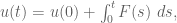
The first step, which is standard in nonlinear evolution equations, is to rewrite the differential equation (1) as an integral equation. Just as the basic ODE

can be rewritten via the fundamental theorem of calculus in the integral form
it turns out that the inhomogeneous wave equation

can be rewritten via the fundamental solution (4) of the homogeneous equation (together with Duhamel’s principle) in the integral form

where  is the solution to the homogeneous wave equation (2) with initial position
  and initial velocity
  (and is given using (4)). [I plan to write more about this formula in a later post, but today I will just treat it as a miraculous identity. I will note however that the formula generalises Newton’s formula
 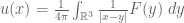 for the standard solution to Poisson’s equation
  .]
.]
Using the fundamental solution, the nonlinear wave equation (1) can be rewritten in integral form as
 (5)
(5)
[Strictly speaking, one needs to first show that the solution exists and is sufficiently smooth before (5) can be rigorously applied, but this turns out to be a routine technical detail and I will not discuss it here.]
John’s argument now exploits a remarkable feature of the fundamental solution of the three-dimensional wave equation, namely that it is non-negative; combining this with the non-negativity of the forcing term  , we see that the integral in (5), that represents the cumulative effect of the nonlinearity, is always non-negative. Thus we have the pointwise inequality
 (6)
(6)
but also we see that any lower bound for u of the form  can be immediately bootstrapped via (5) to a new lower bound
 . (7)
. (7)
This gives a way to iteratively give lower bounds on a solution u, by starting with the lower bound (5) (and computing  explicitly using (4)) and then feeding this bound repeatedly into (7) to see what one gets. (This iteration procedure is closely related to the method of Picard iteration for constructing solutions to nonlinear ODE or PDE, which is still widely used today in the modern theory.)
What will transpire is that this iterative process will yield successively larger lower bounds when  , but will yield successively smaller lower bounds when
  ; this is the main driving force behind John’s theorem. (To actually establish blowup in finite time when , there is an auxiliary step that uses energy inequalities to show that once the solution gets sufficiently large, it will be guaranteed to develop singularities within a finite amount of additional time. To establish global solutions when , one needs to show that the lower bounds constructed by this scheme in fact converge to the actual solution, and establish uniform control on all of these lower bounds.)
The remaining task is a computational one, to evaluate the various lower bounds for u arising from (6) and (7) from some given initial data. In principle, this is just an application of undergraduate several variable calculus, but if one sets about working out the relevant integrals exactly (using polar coordinates, etc.), the computations quickly become tediously complicated. But we don’t actually need exact, closed-form expressions for these integrals; just knowing the order of magnitude of these integrals is enough. For that task, much faster computational techniques are available.
Let’s see how. We begin with the computation of the linear solution . This is given in terms of the initial data  via the formula (4). Now, for the purpose of establishing John’s theorem in the form stated above, we have the freedom to pick the initial data as we please, as long as it is smooth, small, and compactly supported. To make our life easier, we pick initial data with vanishing initial position and non-negative initial velocity, thus
  and
and  ; this eliminates the pesky partial derivative in (4) and makes non-negative. More concretely, let us take

for some fixed non-negative bump function  (the exact form is not relevant) and some small
  , thus the initial velocity has very small amplitude and width. To simplify the notation we shall work with macroscopic values of
  , thus
  , but it will be not hard to see that the arguments below also work for very small (though of course the smaller is, the longer it will take for blowup to occur).
As I said before, we only need an order of magnitude computation. Let us reflect this by describing the initial velocity in fuzzier notation:
 .
.
Geometrically,  has “height”
  on a ball of radius O(1) centred at the origin. We will retain this sort of fuzzy notation throughout the rest of the argument; it is not fully rigorous, but we can always go back and make the computations formal (and much lengthier) after we have performed the quick informal calculations to show the way ahead.
Thus we see from (4) that the linear solution can be expressed somewhat fuzzily in the form
 .
.
Note that the factor  can be discarded for the purposes of order of magnitude computation. Geometrically, the integral is measuring the area of the portion of the sphere
  which intersects the ball
  . A little bit of geometric visualisation will reveal that for large times
  , this portion of the sphere will vanish unless
  , in which case it is a spherical cap of diameter O(1), and thus area O(1). Thus we are led to the back-of-the-envelope computation

with zero when  . (This vanishing outside of a neighbourhood of the light cone
  is a manifestation of the sharp Huygens principle.)
In particular, from (6) we obtain the initial lower bound
 .
.
If we then insert this bound into (7) and discard the linear term (which we already know to be positive, and which we have already “used up” in some sense) we obtain the lower bound

This is a moderately scary looking integral. But we can get a handle on it by first looking at it geometrically. For a fixed point (t,x) in spacetime, the region of integration is the intersection of a backwards light cone  with a thickened forwards light cone
  . If |x| is much larger than t, then these cones will not intersect. If |x| is close to t, the intersection looks complicated, so let us consider the spacelike case when |x| is much less than t, say
  ; we also continue working in the asymptotic regime . In this case, a bit of geometry or algebra shows that the intersection of the two light cones is a two-dimensional ellipsoid in spacetime of radii
  (in particular, its surface area is
  ), and living at times s in the interior of
 ![{}[0,t]](https://s0.wp.com/latex.php?latex=%7B%7D%5B0%2Ct%5D&bg=ffffff&fg=545454&s=0&c=20201002) , thus s and t-s are both comparable to t. Thickening the forward cone, it is then geometrically intuitive that the intersection of the backwards light cone with the thickened forwards light cone is an angled strip around that ellipse of thickness ; thus the total measure of this strip is roughly . Meanwhile, since s and t-s are both comparable to t, the integrand is of magnitude
, thus s and t-s are both comparable to t. Thickening the forward cone, it is then geometrically intuitive that the intersection of the backwards light cone with the thickened forwards light cone is an angled strip around that ellipse of thickness ; thus the total measure of this strip is roughly . Meanwhile, since s and t-s are both comparable to t, the integrand is of magnitude  . Putting all of this together, we conclude that
 (8)
(8)
whenever we are in the interior cone region  .
.
To summarise so far, the linear evolution filled out the light cone  with a decay
  , and then the nonlinearity caused a secondary wave that filled out the interior region
  with a decay
  . We now compute the tertiary wave by inserting the secondary wave bound back into (7), to get

Let us continue working in an interior region, say  . The region of integration is the intersection of the backwards light cone
  with an interior region
  . A brief sketch of the situation reveals that this intersection basically consists of the portion of the backwards light cone in which s is comparable in size to t. In particular, this intersection has a three-dimensional measure of
  , and on the bulk of this intersection, s and t-s are both comparable to t. So we obtain a lower bound
 (9)
(9)
whenever and  .
.
Now we finally see where the condition will come in; if this condition is true, then  is positive, and so the tertiary wave is stronger than the secondary wave, and also situated in essentially the same location of spacetime. This is the beginning of a positive feedback loop; the quaternary wave will be even stronger still, and so on and so forth. Indeed, it is not hard to show that if , then for any constant A, one will have a lower bound of the form
  in the interior of the light cone. This does not quite demonstrate blowup per se – merely superpolynomial growth instead – but actually one can amplify this growth into blowup with a little bit more effort (e.g. integrating (1) in space to eliminate the Laplacian term and investigating the dynamics of the spatial integral
  , taking advantage of finite speed of propagation for this equation, which limits the support of u to the cone
  ). A refinement of these arguments, taking into account more of the components of the various waves in the iteration, also gives blowup for the endpoint .
In the other direction, if , the tertiary wave appears to be smaller than the secondary wave (though to fully check this, one has to compute a number of other components of these waves which we have discarded in the above computations). This sets up a negative feedback loop, with each new wave in the iteration scheme being smaller or decaying faster than the previous, and thus suggests global existence of the solution, at least when the size of the initial data (which was represented by ) was sufficiently small. This heuristic prediction can be made rigorous by controlling these iterates in various function space norms that capture these sorts of decay, but I will not detail them here.
[More generally, any analysis of a semilinear equation that requires one to compute the tertiary wave tends to give conditions on the exponents which are quadratic in nature; if the quaternary wave was involved also, then cubic constraints might be involved, and so forth. In this particular case, an analysis of the primary and secondary waves alone (which would lead just to linear constraints on p) are not enough, because these waves live in very different regions of spacetime and so do not fully capture the feedback mechanism.]
[Update, Oct 27: typo corrected.]
[Update, Nov 6: typo corrected.]


22 comments
Comments feed for this article
26 October, 2007 at 3:03 pm
anon
What happens when u is complex-valued? Most everywhere I see this equation discussed it is real, but most nonlinear wave equations one is treated to the more general case of a complex valued field. Is there some reason that the complex valued case follows immediately or is of no more interest?
27 October, 2007 at 5:44 am
Anonymous
Regarding the “miraculous identity”, what happens when F is not just a function of u, but also of its derivatives? That’s what you typically have to deal with in realistic field theories involving more than one field; F then depends on those other fields, their derivatives, and derivatives of u, all mixed up in various hairraising ways. You might be able to get rid of time derivatives of u by a suitable choice of gauge, but not of spatial derivatives.
27 October, 2007 at 9:47 am
Brian K
For a good discussion of blow up of the Complex KdV equation, and proof of existence beyond blow-up, see Bjorn Birnir’s paper in SIAM Journ of Applied Math, August 1987.
27 October, 2007 at 11:03 am
Shuanglin Shao
I like this trick of back-of-the envelop calculation here: very intuitive but efficient in getting to the point.
I was wondering what cause the eqution (1) so different from the dispersive NLW with nonlinear term instead of
  , where we have so-called critical, subcritical or supercritical phenomena? For instance, according to 1. in the Theorem, even for sufficiently small data, we still have finite time blow up if
  .
.
A typo I found: a little above Eq. (9) in the post, the interior part should be $\latex \{(s,y): s\gg 1; |y|<s/2 \}$.
27 October, 2007 at 2:05 pm
carlbrannen
I appreciate the darker print for the text, thanks Dr. Tao. But now the equations show up in faint print, while the text is dark.
To make LaTeX equations print out in the same dark print requires that one put a gibberish text string just before the final dollar sign. This text defines the foreground and background colors, and also the size of the LaTeX equation. I use &bg=ffffff&fg=000000&s=1 to make things darker and a little larger. To compare the effects for readability: without: and with
  . (Prays briefly that no typos show up in the equations since wordpress won’t let us review comments before submitting.)
28 October, 2007 at 4:46 am
Terence Tao
Regarding extensions of John’s result to other nonlinearities: it is likely that the positive results (global existence for large p) continue to hold in these settings (though the presence of derivatives in the nonlinearity will make things technically more complicated), for instance I think it is known that any nonlinearity which is cubic in u and its first derivatives will lead to global decaying solutions from small data. On the other hand, it is much more difficult to force blowup, even for small p, when the nonlinearity does not have a consistent sign. The focusing nonlinearity is OK since the evolution of this equation will match that of (1) so long as the solution to the latter is non-negative. The defocusing nonlinearity
  is a different matter; here one is guaranteed global existence for all
  even for large (smooth) complex data, basically because of the coercive nature of the conserved energy
  .
.
Scaling considerations (which compare the relative strengths of the coarse and fine scales) here turn out to not be terribly relevant for these small data problems; as the data is smooth and compactly supported, it is almost entirely based in the medium scales, and the data is too small for any cascade of energy from the medium scales into the very fine or very coarse scales to have a significant effect. Instead, it is really the spatial and temporal interactions at the medium scale which are causing the difficulty here (although the secondary and tertiary waves do happen to have significantly lower frequency than the primary).
Dear Carl: unfortunately I do not see a way to automatically insert this string into every LaTeX equation (it seems very unlikely that one can do this via manipulating the CSS, for instance, and there does not appear to be support here for a javascript or macro based solution). Insertion by hand into every equation in every post would be rather impractical for obvious reasons. (A greasemonkey script might work, but I am not adept with these things.)
28 October, 2007 at 3:02 pm
t8m8r
Some blogs seem to show dark equations by default, for example:
29 October, 2007 at 4:00 am
GorDon
Dear Terry,
What do you think about extensions of John’s result which replace
the Laplacian with less smoothing operators? Maybe the form of
the nonlinearity might come into play big time.
29 October, 2007 at 9:36 pm
carlbrannen
Terry, yeah, I put them in “by hand”, or more accurately, using a global search and replace as the last step before publishing. I should add in a keyboard macro, but I hate learning new stuff on computers.
Also, these calculations remind me of some stuff I studied on subharmonics and superharmonics several decades ago. More recently, I’ve played with nonlinear modifications of the Dirac equation.
31 October, 2007 at 4:42 pm
Doug
Hi Terence,
1+sqrt(2)
appears to be equivalent to the relatively periodic
1+2sin(PI/4)
5 November, 2007 at 9:17 pm
Orr
Hello Prof. Tao,
In the paragraph after equation (4), you wrote
“On the other hand, solutions to (2) tend to blow up”
but I think you meant
“On the other hand, solutions to (3) tend to blow up”.
5 November, 2007 at 10:43 pm
Orr
Hello again,
Can you clear up a little the case $p=1$?
First, it seems that your arguments above will work
for $p=1$.
Second, it seems very odd that, as you say, for p=1 there is no
blowup for reasonable data, then for $1 1 + \sqrt{2}$.
Thanks
5 November, 2007 at 10:47 pm
Orr
There was a mistake in my previous comment, should be:
Second, it seems very odd that, as you say, for p=1 there is no
blowup for reasonable data, then for 1 < p 1 + \sqrt{2}.
Sorry and thanks.
6 November, 2007 at 8:54 am
Terence Tao
Dear Orr,
Thanks for the correction. When p=1, the analysis I described above does show that each new iteration of u grows faster than the previous one, and indeed one can soon show that u grows faster than for any fixed A. However, in this case of linear nonlinearity (ugh, you know what I mean), rapid growth does not force finite time blowup, basically because the ODE (3) does not exhibit blowup. Instead, one has exponential growth in time (which can be shown easily using Gronwall’s inequality).
Dear GorDon: When one changes the power of the dispersive term then the fundamental solution is unlikely to stay positive, which makes a direct application of John’s argument difficult. But there may be a way to salvage matters. For instance, subsequent work of Sideris showed that John’s blowup argument can be adapted to higher dimensions; the point being that even though the fundamental solution is no longer positive, certain antiderivatives of that solution remain positive, and this turns out to be enough positivity to coerce rapid growth and then blowup.
6 November, 2007 at 10:19 am
Anonymous
Can anyone inform me about corresponding results or reference when the non-linearity is replaced by u^pf(u,t)? What are the conditions that f should satisfy in order for such an analysis to go through?
6 November, 2007 at 10:30 am
Terence Tao
Dear Anonymous,
There is a substantial literature that follows John’s original 1979 paper, see
http://www.ams.org/mathscinet/search/publications.html?refcit=535704&loc=refcit
I am not sure whether your question is addressed directly, but there are certainly results on blowup on differential inequalities of NLW type which may include some cases of your query as a special case. (There are also results for systems, in the presence of a potential, on manifolds or domains, etc.)
6 November, 2007 at 9:33 pm
deleted
Thanks
15 November, 2007 at 3:58 am
Pedro Lauridsen Ribeiro
A bit dumb (I think) question, related to Anonymous’s question (Nov 6th):
what if the f(x,t) multiplying the nonlinear term is a smooth function of compact support _in spacetime_? Perhaps then one can avoid blowup and have dispersive behaviour of sufiiciently small solutions for rather general nonlinear terms… or not?
15 November, 2007 at 4:35 pm
Terence Tao
Dear Pedro,
If the nonlinearity is compactly supported in time, then after a fixed period of time T the evolution is simply that of the linear wave equation, which cannot blow up. So then the issue is then simply for the solution to outlast the nonlinearity for this fixed amount of time T. By energy methods (using tools such as Gronwall’s inequality) one can show that this can be done if the initial data is small enough (e.g. exponentially small in T will suffice).
7 August, 2008 at 8:22 am
Zarai
Dear Anonymous,
Please Do you have any idea: How prove nonexistence of solutions if we add to the equation (1) the memory term?
2 July, 2009 at 7:30 am
nik
Dear Terry,
it’s a nice argument you presented. However, in the case $ p > 1 + \sqrt{2} $ it is not quite true that “each new wave in the iteration scheme will decay faster”. Actually, each new wave will decay in the the same way as the previous one, with a space-time bound 1/[(1+t+r) (1+|t-r|)^{p-2}]. What makes the scheme convergent is the fact that each next wave gains some extra powers of $ \epsilon $, where $ \epsilon $ is a measure of the smallness of initial data. (If the data is not small enough, there is no convergence.)
I give a very brief explanation of the appearance of the critical value $ p_0 = 1 + \sqrt{2}$ from the convergence point of view ($p>p_0) in appendix of arXiv:0708.2801
All the best.
2 July, 2009 at 7:55 am
Terence Tao
Yes, I did manage to oversimplify in my discussion. If one of these waves enters the interior of the light cone (as was the case in the heuristic discussion), then all subsequent waves caused by that component will decay at increasingly more rapid rates, but yes, if one instead considers the contribution of one of these waves closer to the cone (particularly, closer to the spacetime origin at the vertex of the cone) then they will generate waves of smaller amplitude rather than faster decay. I’ve amended the description slightly to reflect this.