
In the theory of dense graphs on 
Lemma 1 (Regularity lemma, standard version) Let
be a graph on
and
. Then there exists a partition of the vertices
, with
bounded below by
and above by a quantity
depending only on
, obeying the following properties:
- (Equitable partition) For any
, the cardinalities
of
and
differ by at most
.
- (Regularity) For all but at most
pairs
, the portion of the graph
between
-regular in the sense that one has
for any
and
with
, where
is the density of edges between
and
.

This lemma becomes useful in the regime when 

For various technical reasons it is easier to work with a slightly weaker version of the lemma, which allows for the cells 
Lemma 2 (Regularity lemma, weighted version) Let
bounded above by a quantity
depending only on
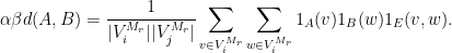
- (Regularity) One has
where the sum is over all pairs
for which
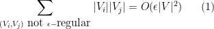
While Lemma 2 is, strictly speaking, weaker than Lemma 1 in that it does not enforce the equitable size property between the atoms, in practice it seems that the two lemmas are roughly of equal utility; most of the combinatorial consequences of Lemma 1 can also be proven using Lemma 2. The point is that one always has to remember to weight each cell 

One disadvantage of the greedy algorithm is that it is not efficient in the limit 


Lemma 3 (Regularity lemma via random neighbourhoods) Let
with the following property: whenever
at random from
uniformly from
vertex cells
(some of which can be empty) generated by the vertex neighbourhoods
for
, will obey the conclusions of Lemma 2 with probability at least
.
Thus, roughly speaking, one can regularise a graph simply by taking a large number of random vertex neighbourhoods, and using the partition (or Venn diagram) generated by these neighbourhoods as the partition. The intuition is that if there is any non-uniformity in the graph (e.g. if the graph exhibits bipartite behaviour), this will bias the random neighbourhoods to seek out the partitions that would regularise that non-uniformity (e.g. vertex neighbourhoods would begin to fill out the two vertex cells associated to the bipartite property); if one takes sufficiently many such random neighbourhoods, the probability that all detectable non-uniformity is captured by the partition should converge to
This fact seems to be reasonably well-known folklore, discovered independently by many authors; it is for instance quite close to the graph property testing results of Alon and Shapira, and also appears implicitly in a paper of Ishigami, as well as a paper of Austin (and perhaps even more implicitly in a paper of myself). However, in none of these papers is the above lemma stated explicitly. I was asked about this lemma recently, so I decided to provide a proof here.
— 1. Warmup: a weak regularity lemma —
To motivate the idea, let’s first prove a weaker but simpler (and more quantitatively effective) regularity lemma, analogous to that established by Frieze and Kannan:
Lemma 4 (Weak regularity lemma via random neighbourhoods) Let
with the following property: whenever
at random, then selects
vertices
uniformly from
vertex cells
(some of which can be empty) generated by the vertex neighbourhoods
for
, obey the following property with probability at least
, the number of edges
connecting

This weaker lemma only lets us count “macroscopic” edge densities 

Let’s now prove this lemma. Fix 


We will use the trick of turning sets into functions, and view the graph as a function 


We give 


one can interpret this as the mean square of the edge densities 

for all 


telescopes to be 


Suppose

where

and

We now assert that the partition 

Lemma 5 (
is structured)
.
Proof: This is clear from construction.

Lemma 6 (
is pseudorandom) The expression
is of size
.

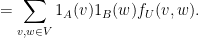
Proof: The left-hand side can be rewritten as

Observe that the function 


Applying Cauchy-Schwarz, one can bound this by

But from Pythagoras we have

and so the claim follows from (3) and another application of Cauchy-Schwarz.
Now we can prove Lemma 4. Observe that

Applying Cauchy-Schwarz twice in 


— 2. Strong regularity via random neighbourhoods —
We now prove Lemma 3, which of course implies Lemma 2.
Fix 

Now let 


telescopes to be 
Assume that 


Fix this

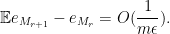
so by Markov’s inequality, with probability

and also obey the conditional expectation bound

Assume that this is the case. We split

where


We now assert that the partition 
Lemma 7 (
.
Proof: This is clear from construction.
 .
.
Proof: This follows from (4) and Pythagoras’ theorem.
Lemma 9 (
is of size
.
Proof: This follows by repeating the proof of Lemma 6, but using (5) instead of (3).
Now we verify the regularity.
First, we eliminate small atoms: the pairs 


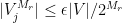

Now, let 


then
We divide 
The contribution of 
The contribution of

Using Lemma 8 and Chebyshev’s inequality, we see that the pairs 


Finally, the contribution of
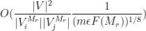
which by (6) is bounded by

This can be made 


which (since 
Remark 1 Of course, this argument gives tower-exponential bounds (as
Remark 2 One can take the partition induced by random neighbourhoods here and carve it up further to be both equitable and (mostly) regular, thus recovering a proof of Lemma 1, by following the arguments in this paper of mine. Of course, when one does so, one no longer has a partition created purely from random neighbourhoods, but it is pretty clear that one is not going to be able to make an equitable partition just from boolean operations applied to a few random neighbourhoods.

9 comments
Comments feed for this article
27 April, 2009 at 9:09 am
Asaf
Hi Terry,
Such an O(n) algorithm appears (explicitly) in the following paper of mine with Fischer and Matsliach.
Click to access regalg.pdf
That algorithm actually has the added advantage of being able to find (more or less) the smallest regular partition in the input.
27 April, 2009 at 10:31 am
Terence Tao
Dear Asaf: thanks for the reference! It again seems to be slightly different from the random neighbourhoods algorithm (which is a O(1) algorithm rather than O(n), but only defines the partition implicitly and does not make it equitable) but certainly in the same spirit.
27 April, 2009 at 8:11 pm
Anup
Hi Terry, for Lemma 2, do you want to allow i=j in the sum?
Otherwise it seems that partitioning the graph into one part V1 = V, would trivially satisfy the conclusions of the lemma.
[Hmm, you’re right. Thanks for the correction! – T.]
8 May, 2009 at 8:14 pm
Szemeredi’s regularity lemma via the correspondence principle « What’s new
[…] math.PR | Tags: correspondence principle, szemeredi regularity lemma | by Terence Tao In a previous post, we discussed the Szemerédi regularity lemma, and how a given graph could be regularised by […]
5 August, 2009 at 5:17 pm
Moser’s entropy compression argument « What’s new
[…] is often referred to as the “index”). These examples are related; see this blog post for further discussion. The general strategy here is to keep looking for useful pieces of energy […]
24 December, 2011 at 11:31 am
Szemerédi’s regularity lemma « Disquisitiones Mathematicae
[…] the book The probabilistic method of Alon and Spencer, the survey of Komlós and M. Simonovits and Tao’s perspective via random partitions. Merry Christmas!! Share this:TwitterLike this:LikeBe the first to like this […]
3 December, 2012 at 5:35 pm
The spectral proof of the Szemeredi regularity lemma « What’s new
[…] proofs of this lemma, which is actually not that difficult to establish; see for instance these previous blog posts for some examples. In this post I would like to record one further proof, based on the […]
29 May, 2014 at 7:19 pm
deep
Hi Terry,
I wanted to make sense of Szemerédi regularity lemma (SRL) for Erdős–Rényi random graph G(n,p).
If I understood correctly the SRL states that any random dense graph (the adjacency matrix) can be “approximately” partitioned into block-diagonal structures (after proper rearrangement) .
Lets generate G(n=10000,p=.1), a dense random network butthe corresponding adjacency matrix A it can NOT be represented as a block-diagonal form (whatever rearrangement we do). Then my question is, how to interpret SRL in thisset-up ? What I’m missing ?
Thank you so much for your time and apology for my ignorance.
30 May, 2014 at 7:56 am
Terence Tao
Actually, the regularity lemma asserts (roughly speaking) that any dense graph can be approximately partitioned, after rearrangement, into blocks, in which the graph behaves like a random graph in each block (of some density p which need not be 0 or 1, but can also be something in between). So, if one starts with an Erdős–Rényi graph, one is already done: we only need one block, because the graph already exhibits random behaviour in that block.
To put it another way, the regularity lemma tells us that every large dense adjacency matrix is in some sense a “combination” of a bounded rank matrix (which divides up into a bounded number of blocks) and a random matrix; the “block-diagonal” matrices and the Erdős–Rényi matrices reflect the two possible extremes of behaviour, and every other graph is in some sense a mixture of these two extremes.