The Riemann zeta function  , defined for
  by
by

and then continued meromorphically to other values of  by analytic continuation, is a fundamentally important function in analytic number theory, as it is connected to the primes
  via the Euler product formula
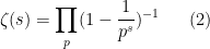
(for  , at least), where
  ranges over primes. (The equivalence between (1) and (2) is essentially the generating function version of the fundamental theorem of arithmetic.) The function
  has a pole at
  and a number of zeroes
  . A formal application of the factor theorem gives

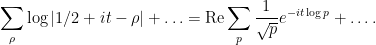
where ranges over zeroes of , and we will be vague about what the  factor is, how to make sense of the infinite product, and exactly which zeroes of are involved in the product. Equating (2) and (3) and taking logarithms gives the formal identity

using the Taylor expansion

and differentiating the above identity in yields the formal identity
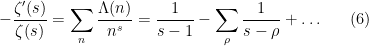
where  is the von Mangoldt function, defined to be
  when
when  is a power of a prime , and zero otherwise. Thus we see that the behaviour of the primes (as encoded by the von Mangoldt function) is intimately tied to the distribution of the zeroes . For instance, if we knew that the zeroes were far away from the axis
  , then we would heuristically have
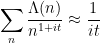
for real  . On the other hand, the integral test suggests that
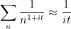
and thus we see that  and
and  have essentially the same (multiplicative) Fourier transform:

Inverting the Fourier transform (or performing a contour integral closely related to the inverse Fourier transform), one is led to the prime number theorem
In fact, the standard proof of the prime number theorem basically proceeds by making all of the above formal arguments precise and rigorous.
Unfortunately, we don’t know as much about the zeroes of the zeta function (and hence, about the function itself) as we would like. The Riemann hypothesis (RH) asserts that all the zeroes (except for the “trivial” zeroes at the negative even numbers) lie on the critical line  ; this hypothesis would make the error terms in the above proof of the prime number theorem significantly more accurate. Furthermore, the stronger GUE hypothesis asserts in addition to RH that the local distribution of these zeroes on the critical line should behave like the local distribution of the eigenvalues of a random matrix drawn from the gaussian unitary ensemble (GUE). I will not give a precise formulation of this hypothesis here, except to say that the adjective “local” in the context of distribution of zeroes means something like “at scale
  when
when  “.
“.
Nevertheless, we do know some reasonably non-trivial facts about the zeroes and the zeta function , either unconditionally, or assuming RH (or GUE). Firstly, there are no zeroes for (as one can already see from the convergence of the Euler product (2) in this case) or for (this is trickier, relying on (6) and the elementary observation that

is non-negative for  and
and  ); from the functional equation

(which can be viewed as a consequence of the Poisson summation formula, see e.g. my blog post on this topic) we know that there are no zeroes for  either (except for the trivial zeroes at negative even integers, corresponding to the poles of the Gamma function). Thus all the non-trivial zeroes lie in the critical strip
  .
.
We also know that there are infinitely many non-trivial zeroes, and can approximately count how many zeroes there are in any large bounded region of the critical strip. For instance, for large  , the number of zeroes in this strip with
  is
is  . This can be seen by applying (6) to
  (say); the trivial zeroes at the negative integers end up giving a contribution of to this sum (this is a heavily disguised variant of Stirling’s formula, as one can view the trivial zeroes as essentially being poles of the Gamma function), while the
  and terms end up being negligible (of size
  ), while each non-trivial zero contributes a term which has a non-negative real part, and furthermore has size comparable to if . (Here I am glossing over a technical renormalisation needed to make the infinite series in (6) converge properly.) Meanwhile, the left-hand side of (6) is absolutely convergent for
  and of size , and the claim follows. A more refined version of this argument shows that the number of non-trivial zeroes with
  is
is  , but we will not need this more precise formula here. (A fair fraction – at least 40%, in fact – of these zeroes are known to lie on the critical line; see this earlier blog post of mine for more discussion.)
Another thing that we happen to know is how the magnitude  of the zeta function is distributed as
  ; it turns out to be log-normally distributed with log-variance about
  . More precisely, we have the following result of Selberg:
Theorem 1 Let be a large number, and let be chosen uniformly at random from between and  (say). Then the distribution of
  converges (in distribution) to the normal distribution
  .
.
To put it more informally,  behaves like
  plus lower order terms for “typical” large values of . (Zeroes of are, of course, certainly not typical, but one can show that one can usually stay away from these zeroes.) In fact, Selberg showed a slightly more precise result, namely that for any fixed
  , the
, the  moment of converges to the moment of .
Remarkably, Selberg’s result does not need RH or GUE, though it is certainly consistent with such hypotheses. (For instance, the determinant of a GUE matrix asymptotically obeys a remarkably similar log-normal law to that given by Selberg’s theorem.) Indeed, the net effect of these hypotheses only affects some error terms in of magnitude , and are thus asymptotically negligible compared to the main term, which has magnitude about  . So Selberg’s result, while very pretty, manages to finesse the question of what the zeroes of are actually doing – he makes the primes do most of the work, rather than the zeroes.
Selberg never actually published the above result, but it is reproduced in a number of places (e.g. in this book by Joyner, or this book by Laurincikas). As with many other results in analytic number theory, the actual details of the proof can get somewhat technical; but I would like to record here (partly for my own benefit) an informal sketch of some of the main ideas in the argument.
— 1. Informal overview of argument —
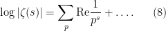
The first step is to get a usable (approximate) formula for  . On the one hand, from the second part of (4) one has

This formula turns out not to be directly useful because it requires one to know much more about the distribution of the zeroes than we currently possess. On the other hand, from the first part of (4) and (5) one also has the formula
This formula also turns out not to be directly useful, because it requires one to know much more about the distribution of the primes than we currently possess.
However, it turns out that we can “split the difference” between (7), (8), and get a formula for  which involves some zeroes and some primes , in a manner that one can control them both. Roughly speaking, the formula looks like this:

for  and
and  , where
  is a small parameter that we can choose (e.g.
  ); thus we have localised the prime sum to the primes of size
  , and the zero sum to those zeroes at a distance from . (This is an oversimplification; there is a “tail” coming from those zeroes that are more distant from than , and also one has to smooth out the sum in a little bit, and allow the implied constants in the
  notation to depend on , but let us ignore these technical issues here, as well as the issue of what exactly is hiding in the error.)
It turns out that all of these expressions can be controlled. The error term coming from the zeroes (as well as the error term) turn out to be of size for most values of , so are a lower order term. (As mentioned before, it is this error term that would be better controlled if one had RH or GUE, but this is not necessary to establish Selberg’s result.) The main term is the one coming from the primes.
We can heuristically argue as follows. The expression 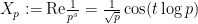 , for ranging between and , is a random variable of mean zero and variance approximately
  (if
(if  and is small). Making the heuristic assumption that the
  behave as if they were independent, the central limit theorem then suggests that the sum
  should behave like a normal distribution of mean zero and variance
  . But the claim now follows from the classical estimate
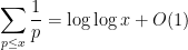
(which follows from the prime number theorem, but can also be deduced from the formula (8) for  , using the fact that has a simple pole at ).
To summarise, there are three main tasks to establish Selberg’s theorem:
- Establish a formula along the lines of (9);
- Show that the error terms arising from zeroes are on the average;
- Justify the central limit calculation for
 .
.
I’ll now briefly talk (informally) about each of the three steps in turn.
— 2. The explicit formula —
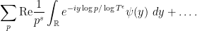
To get a formula such as (9), the basic strategy is to take a suitable average of the formula (7) and the formula (8). Traditionally, this is done by contour integration; however, I prefer (perhaps idiosyncratically) to take a more Fourier-analytic perspective, using convolutions rather than contour integrals. (The two approaches are largely equivalent, though.) The basic point is that the imaginary part  of the zeroes inhabits the same space as the imaginary part
  of the variable, which in turn is the Fourier analytic dual of the variable that the logarithm of the primes live in; this can be seen by writing (7), (8) in a more Fourier-like manner as
(These sorts of Fourier-analytic connections are often summarised by the slogan “the zeroes of the zeta function are the music of the primes”.) The uncertainty principle then predicts that localising to the scale  should result in blurring out the zeroes at scale
  , which is where (9) is going to come from.
Let’s see how this idea works in practice. We consider a convolution of the form

where  is some bump function with total mass ; informally, this is averaged out in the vertical direction at scale
  (we allow implied constants to depend on ).
We can express (10) in two different ways, one using (7), and one using (8). Let’s look at (7) first. If one modifies by , then the quantity  doesn’t fluctuate very much, unless is within of , in which case it can move by about
  . As a consequence, we see that

when  , and
, and

The quantity  also doesn’t move very much by this shift (we are assuming the imaginary part of to be large). Inserting these facts into (7), we thus see that (10) is (heuristically) equal to

Now let’s compute (10) using (8) instead. Writing  , we express (10) as
Introducing the Fourier transform  of , one can write this as

Now we took to be a bump function, so its Fourier transform should also be like a bump function (or perhaps a Schwartz function). As a first approximation, one can thus think of  as a smoothed truncation to the region
  , thus the
  weight is morally restricting to the region . Thus we (morally) can express (10) as
Comparing this with the other formula (11) we have for (10), we obtain (9) as required (formally, at least).
— 3. Controlling the zeroes —
Next, we want to show that the quantity
is on the average, when  and is chosen uniformly at random from to .
For this, we can use the first moment method. For each zero , let  be the random variable which equals
  when
when  and zero otherwise, thus we are trying to control the expectation of
  . The only zeroes which are relevant are those which are of size
  , and we know that there are
  of these (indeed, we have an even more precise formula, as remarked earlier). On the other hand, a randomly chosen has a probability of
  of falling within of , and so we expect each to have an expected value of
  . (The logarithmic factor in the definition of turns out not to be an issue, basically because
  is locally integrable.) By linearity of expectation, we conclude that has expectation
  , and the claim follows.
Remark 1 One can actually do a bit better than this, showing that higher order moments of are also , by using a variant of (9) together with the moment bounds in the next section; but we will not need that refinement here.
— 4. The central limit theorem —
Finally, we have to show that behaves like a normal distribution, as predicted by the central limit theorem heuristic. The key is to show that the behave “as if” they were jointly independent. In particular, as the all have mean zero, one would like to show that products such as
have a negligible expectation as long as at least one of the primes in  occurs at most once. Once one has this (as well as a similar formula for the case when all primes appear at least twice), one can then do a standard moment computation of the moment
  and verify that this moment then matches the answer predicted by the central limit theorem, which by standard arguments (involving the Weierstrass approximation theorem) is enough to establish the distributional law. Note that to get close to the normal distribution by a fixed amount of accuracy, it suffices to control a bounded number of moments, which ultimately means that we can treat
  as being bounded,
  .
.
If we expand out the product (12), we get

Using the product formula for cosines (or Euler’s formula), the product of cosines here can be expressed as a linear combination of cosines  , where the frequency
  takes the form

Thus, is the logarithm of a rational number, whose numerator and denominator are the product of some of the . Since all the  are at most
  , we see that the numerator and denominator here are at most
  .
.
Now for the punchline. If there is a prime in that appears only once, then the numerator and denominator cannot fully cancel, by the fundamental theorem of arithmetic. Thus cannot be  . Furthermore, since the denominator is at most , we see that must stay away from by a distance of about
  or more, and so has a wavelength of at most
  . On the other hand, ranges between and . If is fixed and is small enough (much smaller than
  ), we thus see that the average value of between and is close to zero, and so (12) does indeed have negligible expectation as claimed. (A similar argument lets one compute the expectation of (12) when all primes appear at least twice.)
Remark 2 A famous theorem of Erdös and Kac gives a normal distribution for the number of prime factors of a large number , with mean  and variance . One can view Selberg’s theorem as a sort of Fourier-analytic variant of the Erdös-Kac theorem.
Remark 3 The Fourier-like correspondence between zeroes of the zeta function and primes can be used to convert statements about zeroes, such as the Riemann hypothesis and the GUE hypothesis, into equivalent statements about primes. For instance, the Riemann hypothesis is equivalent to having the square root error term

in the prime number theorem holding asymptotically as  for all
  and all intervals
 ![{[x,x+y]}](https://s0.wp.com/latex.php?latex=%7B%5Bx%2Cx%2By%5D%7D&bg=ffffff&fg=000000&s=0&c=20201002) which are large in the sense that
which are large in the sense that  is comparable to
  . Meanwhile, the pair correlation conjecture (the simplest component of the GUE hypothesis) is equivalent (on RH) to the square root error term holding (with the expected variance) for all and almost all intervals which are short in the sense that
  for some small (fixed)
  . (This is a rough statement; a more precise formulation can be found in this paper of Goldston and Montgomery.) It seems to me that reformulation of the full GUE hypothesis in terms of primes should be similar, but would assert that the error term in the prime number theorem (as well as variants of this theorem for almost primes) in short intervals enjoys the expected normal distribution; I don’t know of a precise formulation of this assertion, but calculations in this direction lie in this paper of Bogomolny and Keating.)


24 comments
Comments feed for this article
12 July, 2009 at 9:41 pm
Anonymous
Dear Prof. Tao,
Thank you very much for the post.
Could you please recommend an introductory level analytic number theory book?
thanks
12 July, 2009 at 11:20 pm
Emmanuel Kowalski
The connection between Selberg’s central limit theorem for zeta(s) and the Erdös-Kác theorem is quite interesting; as I’ve discussed recently (based on joint work with A. Nikgehbali and J. Jacod), they can both be interpreted as renormalized consequences of un-normalized limiting behavior of the relevant characteristic functions/Fourier transforms (although for zeta(s), this is only conditional, depending on a suitable form of the Random Matrix correspondance).
One difference is that the case of zeta(s) involves unitary matrices and gaussian variables, while the Erdös-Kác theorem involves permutations and Poisson variables. (See this preprint).
13 July, 2009 at 5:44 pm
Anonymous
There’s a small typo in ” that does appears only once”. [Corrected, thanks -T.]
13 July, 2009 at 7:32 pm
Anonymous
I have a question about the truncation in (9). Isn’t it sub-optimal? We are truncating in physical space at while in frequency space at
  . But
. But  is, at least in most results regarding the zeta function, far away from
  . By the uncertainty principle shouldn’t we be able to truncate at
  without much (any?) impact on the tail terms in frequency space? Of course, you could argue that we aren’t going to improve the conclusion of the theorem so why does it matter, but it struck me as odd.
13 July, 2009 at 7:54 pm
Anonymous
Oh, i think i see, we are realy localizing at .
.
14 July, 2009 at 4:51 am
Anonymous
This question my be sightly off comment but out of curiosity…
A question regarding the Zeros of the Riemann’s Zeta.
I believe that Hardy proved the Riemann’s conjecture for an countable number of zeros.
I have been told that this has been improved so that the number of zeros is commensurate with the continuum!
Is this correct!??? If so please can you give any references!
Thanks in advance
6 August, 2009 at 12:33 am
hezhigang
to infinite set, same cardinality can not imply equivalent.
card{n^2|n∈N}=card{n|n∈N}, but their elements are different in much detail.
14 July, 2009 at 8:03 am
Alex Kontorovich
Dear Terry,
Thanks for the interesting post. Since you also recently posted about Benford’s law, I wanted to mention a paper with Steve (J.) Miller:
http://arxiv.org/abs/math.NT/0412003
in which we show that the values of $L$-functions near the critical line exhibit Benford behavior, using generalizations of Selberg’s theorem. In the same paper we show that iterates in the 3x+1 problem are also Benford; there is also a subsequent paper of Lagarias and Sound on the matter:
http://arxiv.org/abs/math/0509175
Best, Alex
14 July, 2009 at 3:18 pm
Matthew Emerton
Dear Anonymous (at 4:51 am, July 14),
Any non-zero meromorphic function has only countably many zeroes, since the zeroes are a discrete set. In particular, the zeta function has only countably
many zeroes on the critical line.
Hardy proved that an infinite number of zeroes lie on the critical line, and this
result was later improved (by Selberg) to show that a positive proportion of zeroes lies on the line.
15 July, 2009 at 7:03 am
Anonymous
Hi everyone!
Slightly off topic…
There appears to be a revised version of some papers on the Archive
A Proof of the Density Hypothesis
http://arxiv.org/abs/0810.2103
Yuan-You Fu-Rui Cheng
Anything to this
26 February, 2010 at 6:25 am
Anonymous
The revised version has been posted on Feb. 26, 2010.
13 December, 2012 at 7:59 pm
Anonymous
http://arxiv.org/abs/0810.2103
Yuanyou Cheng and Sergio Albeverio
17 July, 2009 at 1:57 am
zhiganghe
some naive question:
in formula (3), is {\rho} contains both trivial zeroes and complex zeroes?
why 1/(s-1)?
I understand it as s=1 is pole of zeta.
Lars V. Ahlfors said in Complex Analysis’ preface that ues of words ‘clearly’, ‘obviously’, ‘evidently’ to test the reader’s understanding.
as a layman to math, I can understand few lines of such professional blog
18 July, 2009 at 5:59 pm
Anonymous
Thank you for presenting this.
Minor detail:
Are there a few missing minus signs? For example, it’s minus the logarithmic derivative of zeta which gives the von Mangoldt function. I think this applies to the left hand sides of equations (4), (5) and (7) — maybe more?
[Corrected, thanks – T.]
21 July, 2009 at 1:44 am
Sika
Dear professor, I believe that you have error/typo in remark 2.
sqrt(log log (n)) is standard deviation, not variance, for the number of prime factors of a large number n. [Corrected, thanks – T.]
Regards, sika
24 July, 2009 at 2:57 am
Michael Nielsen » Biweekly links for 07/24/2009
[…] Selberg’s limit theorem for the Riemann zeta function on the critical line « What’s new […]
7 August, 2009 at 5:59 am
Valentina
Dear Prof. Tao,
Thank you very much for the notes!
31 January, 2010 at 7:40 am
Andrea Alu
Terry: congratulations on the King Faisal award. Will you be picking it up?
7 February, 2010 at 12:06 pm
Anonymous
You wrote: ‘(this is a heavily disguised variant of Stirling’s formula, as one can view the trivial zeroes as essentially being zeroes of the Gamma function)’
Did you mean ‘poles of the Gamma function’? (since the Gamma function doesn’t have zeros)
[Corrected, thanks – T.]
25 June, 2010 at 6:44 pm
The uncertainty principle « What’s new
[…] e.g. this blog post of mine for more discussion). Using such formulae, one can relate the zeroes of the zeta function in the […]
21 December, 2010 at 6:15 pm
Duy
Dear Prof. Tao,
I tried to find the proof of Selberg’s CLT and I found your interesting discussion here. Thank you very much. Actually, I have the book of Laurincikas but it is not so clear for me. Could you tell me where I can find the complete argument as you post here?
30 October, 2014 at 2:29 am
polishchuk
Reading the work of “N. Levinson, More than one third of the zeros of Riemann’s zeta-function are on a=1/2 (1974)” I thought that for molifier Selberg can apply the Riemann hypothesis and later use this new molifier. Terence Tao as you think it may affect the number of zeros or not? Thank you..
4 June, 2017 at 9:55 am
David Cole
FYI: https://www.researchgate.net/post/Does_the_nth_nontrivial_simple_zero_of_the_Riemann_zeta_function_indicate_the_nth_prime_p_n_occurs_as_a_prime_factor_in_all_multiples_of_p_n.
28 September, 2019 at 3:09 pm
Alex
Dear Professor Tao,
Do we have any existing results in literature in which the Martingale Central Limit Theorem has the limit as a stable distribution instead of Normal distribution ?