[This blog post was written jointly by Terry Tao and Will Sawin.]
In the previous blog post, one of us (Terry) implicitly introduced a notion of rank for tensors which is a little different from the usual notion of tensor rank, and which (following BCCGNSU) we will call “slice rank”. This notion of rank could then be used to encode the Croot-Lev-Pach-Ellenberg-Gijswijt argument that uses the polynomial method to control capsets.
Afterwards, several papers have applied the slice rank method to further problems – to control tri-colored sum-free sets in abelian groups (BCCGNSU, KSS) and from there to the triangle removal lemma in vector spaces over finite fields (FL), to control sunflowers (NS), and to bound progression-free sets in  -groups (P).
In this post we investigate the notion of slice rank more systematically. In particular, we show how to give lower bounds for the slice rank. In many cases, we can show that the upper bounds on slice rank given in the aforementioned papers are sharp to within a subexponential factor. This still leaves open the possibility of getting a better bound for the original combinatorial problem using the slice rank of some other tensor, but for very long arithmetic progressions (at least eight terms), we show that the slice rank method cannot improve over the trivial bound using any tensor.
It will be convenient to work in a “basis independent” formalism, namely working in the category of abstract finite-dimensional vector spaces over a fixed field  . (In the applications to the capset problem one takes
  to be the finite field of three elements, but most of the discussion here applies to arbitrary fields.) Given
  such vector spaces
  , we can form the tensor product
  , generated by the tensor products
  with
with  for
for  , subject to the constraint that the tensor product operation
  is multilinear. For each
  , we have the smaller tensor products
  , as well as the
  tensor product
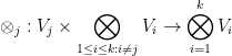
defined in the obvious fashion. Elements of of the form  for some
  and
and  will be called rank one functions, and the slice rank (or rank for short)
  of an element
  of is defined to be the least nonnegative integer
  such that is a linear combination of rank one functions. If are finite-dimensional, then the rank is always well defined as a non-negative integer (in fact it cannot exceed
  . It is also clearly subadditive:

For  , is
, is  when is zero, and
  otherwise. For
  , is the usual rank of the
  -tensor
  (which can for instance be identified with a linear map from
  to the dual space
  ). The usual notion of tensor rank for higher order tensors uses complete tensor products , as the rank one objects, rather than , giving a rank that is greater than or equal to the slice rank studied here.
From basic linear algebra we have the following equivalences:
Lemma 1 Let be finite-dimensional vector spaces over a field , let be an element of  , and let be a non-negative integer. Then the following are equivalent:
Proof: The equivalence of (i) and (ii) is clear from definition. To get from (ii) to (iii) one simply takes  to be the span of the
  , and conversely to get from (iii) to (ii) one takes the to be a basis of the and computes
  by using a basis for the tensor product
 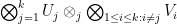 consisting entirely of functions of the form
  for various
  . To pass from (iii) to (iv) one takes
  to be the annihilator
  of , and conversely to pass from (iv) to (iii).
One corollary of the formulation (iv), is that the set of tensors of slice rank at most is Zariski closed (if the field  is algebraically closed), and so the slice rank itself is a lower semi-continuous function. This is in contrast to the usual tensor rank, which is not necessarily semicontinuous.
Corollary 2 Let  be finite-dimensional vector spaces over an algebraically closed field . Let be a nonnegative integer. The set of elements of of slice rank at most is closed in the Zariski topology.
Proof: In view of Lemma 1(i and iv), this set is the union over tuples of integers  with
with  of the projection from
  of the set of tuples
  with
with  orthogonal to
  , where
  is the Grassmanian parameterizing
  -dimensional subspaces of
  .
.
One can check directly that the set of tuples with orthogonal to is Zariski closed in  using a set of equations of the form
 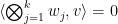 locally on
  . Hence because the Grassmanian is a complete variety, the projection of this set to is also Zariski closed. So the finite union over tuples of these projections is also Zariski closed.
We also have good behaviour with respect to linear transformations:
Lemma 3 Let  be finite-dimensional vector spaces over a field , let be an element of , and for each , let
  be a linear transformation, with
  the tensor product of these maps. Then

Furthermore, if the  are all injective, then one has equality in (2).
Thus, for instance, the rank of a tensor  is intrinsic in the sense that it is unaffected by any enlargements of the spaces .
Proof: The bound (2) is clear from the formulation (ii) of rank in Lemma 1. For equality, apply (2) to the injective , as well as to some arbitrarily chosen left inverses  of the .
Computing the rank of a tensor is difficult in general; however, the problem becomes a combinatorial one if one has a suitably sparse representation of that tensor in some basis, where we will measure sparsity by the property of being an antichain.
Proposition 4 Let be finite-dimensional vector spaces over a field . For each , let  be a linearly independent set in
  indexed by some finite set
  . Let
. Let  be a subset of
  .
.
Let  be a tensor of the form

where for each  ,
,  is a coefficient in . Then one has
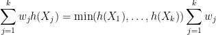

where the minimum ranges over all coverings of by sets  , and
, and  for
for  are the projection maps.
Now suppose that the coefficients are all non-zero, that each of the are equipped with a total ordering  , and
, and  is the set of maximal elements of , thus there do not exist distinct
  ,
,  such that
  for all . Then one has

In particular, if is an antichain (i.e. every element is maximal), then equality holds in (4).
Proof: By Lemma 3 (or by enlarging the bases  ), we may assume without loss of generality that each of the is spanned by the . By relabeling, we can also assume that each is of the form
with the usual ordering, and by Lemma 3 we may take each to be  , with
  the standard basis.
Let denote the rank of . To show (4), it suffices to show the inequality

for any covering of by . By removing repeated elements we may assume that the  are disjoint. For each , the tensor

can (after collecting terms) be written as

for some  . Summing and using (1), we conclude the inequality (6).
Now assume that the are all non-zero and that is the set of maximal elements of . To conclude the proposition, it suffices to show that the reverse inequality

holds for some covering . By Lemma 1(iv), there exist subspaces of  whose dimension
  sums to
such that is orthogonal to  .
.
Let . Using Gaussian elimination, one can find a basis  of whose representation in the standard dual basis
  of is in row-echelon form. That is to say, there exist natural numbers

such that for all  ,
,  is a linear combination of the dual vectors
  , with the
  coefficient equal to one.
We now claim that  is disjoint from . Suppose for contradiction that this were not the case, thus there exists
  for each such that

As is the set of maximal elements of , this implies that
for any tuple  other than
  . On the other hand, we know that
  is a linear combination of
  , with the
  coefficient one. We conclude that the tensor product
  is equal to

plus a linear combination of other tensor products  with
with  not in . Taking inner products with (3), we conclude that
  , contradicting the fact that is orthogonal to
  . Thus we have disjoint from .
For each , let  denote the set of tuples in with
  not of the form
  . From the previous discussion we see that the cover , and we clearly have
  , and hence from (8) we have (7) as claimed.
As an instance of this proposition, we recover the computation of diagonal rank from the previous blog post:
Example 5 Let be finite-dimensional vector spaces over a field for some  . Let be a natural number, and for , let
  be a linearly independent set in . Let
  be non-zero coefficients in . Then

has rank . Indeed, one applies the proposition with  all equal to
  , with the diagonal in ; this is an antichain if we give one of the
  the standard ordering, and another of the the opposite ordering (and ordering the remaining arbitrarily). In this case, the
  are all bijective, and so it is clear that the minimum in (4) is simply .
The combinatorial minimisation problem in the above proposition can be solved asymptotically when working with tensor powers, using the notion of the Shannon entropy  of a discrete random variable
  .
.
Proposition 6 Let be finite-dimensional vector spaces over a field . For each , let be a linearly independent set in indexed by some finite set . Let be a non-empty subset of .
Let be a tensor of the form (3) for some coefficients . For each natural number  , let
, let  be the tensor power of copies of , viewed as an element of
  . Then

as  , where
  is the quantity

and  range over the random variables taking values in .
Now suppose that the coefficients are all non-zero and that each of the are equipped with a total ordering . Let be the set of maximal elements of in the product ordering, and let  where range over random variables taking values in . Then

as . In particular, if the maximizer in (10) is supported on the maximal elements of (which always holds if is an antichain in the product ordering), then equality holds in (9).
Proof:
It will suffice to show that

as , where  is the projection map. Then the same thing will apply to and
  . Then applying Proposition 4, using the lexicographical ordering on
  and noting that, if are the maximal elements of , then
  are the maximal elements of
  , we obtain both (9) and (11).
We first prove the lower bound. By compactness (and the continuity properties of entropy), we can find a random variable taking values in such that

Let  be a small positive quantity that goes to zero sufficiently slowly with . Let
  denote the set of all tuples
  in that are within
  of being distributed according to the law of , in the sense that for all
  , one has

By the asymptotic equipartition property, the cardinality of  can be computed to be

if goes to zero slowly enough. Similarly one has

and for each  , one has

Now let  be an arbitrary covering of . By the pigeonhole principle, there exists such that
and hence by (14), (15)

which by (13) implies that

noting that the  factor can be absorbed into the
  error). This gives the lower bound in (12).
Now we prove the upper bound. We can cover by  sets of the form
  for various choices of random variables taking values in . For each such random variable , we can find such that
  ; we then place all of in . It is then clear that the cover and that

for all  , giving the required upper bound.
It is of interest to compute the quantity in (10). We have the following criterion for when a maximiser occurs:
Proposition 7 Let be finite sets, and  be non-empty. Let be the quantity in (10). Let be a random variable taking values in , and let
  denote the essential range of , that is to say the set of tuples
  such that
  is non-zero. Then the following are equivalent:
Furthermore, when (i) and (ii) holds, one has
Proof: We first show that (i) implies (ii). The function  is concave on
 ![{[0,1]}](https://s0.wp.com/latex.php?latex=%7B%5B0%2C1%5D%7D&bg=ffffff&fg=000000&s=0&c=20201002) . As a consequence, if we define
. As a consequence, if we define  to be the set of tuples
  such that there exists a random variable
  taking values in with
  , then is convex. On the other hand, by (10), is disjoint from the orthant
  . Thus, by the hyperplane separation theorem, we conclude that there exists a half-space

where  are reals that are not all zero, and
  is another real, which contains
  on its boundary and in its interior, such that avoids the interior of the half-space. Since is also on the boundary of , we see that the
  are non-negative, and that
  whenever
  .
.
By construction, the quantity

is maximised when  . At this point we could use the method of Lagrange multipliers to obtain the required constraints, but because we have some boundary conditions on the (namely, that the probability that they attain a given element of has to be non-negative) we will work things out by hand. Let
  be an element of , and
  an element of
  . For
. For  small enough, we can form a random variable taking values in , whose probability distribution is the same as that for except that the probability of attaining
  is increased by , and the probability of attaining is decreased by . If there is any
  for which
 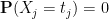 and
and  , then one can check that

for sufficiently small , contradicting the maximality of ; thus we have  whenever . Taylor expansion then gives

for small , where
and similarly for  . We conclude that
  for all
  and
and  , thus there exists a quantity
  such that
  for all , and
  for all . By construction must be nonnegative. Sampling using the distribution of , one has

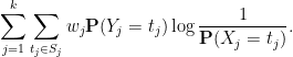
almost surely; taking expectations we conclude that
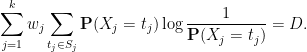
The inner sum is  , which equals when is non-zero, giving (17).
Now we show conversely that (ii) implies (i). As noted previously, the function is concave on , with derivative  . This gives the inequality

for any  (note the right-hand side may be infinite when
  and
and  ). Let be any random variable taking values in , then on applying the above inequality with
  and
and  , multiplying by , and summing over and
  gives
gives

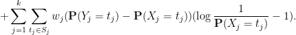
By construction, one has
and

so to prove that  (which would give (i)), it suffices to show that

or equivalently that the quantity

is maximised when . Since

it suffices to show this claim for the quantity
One can view this quantity as

By (ii), this quantity is bounded by , with equality if is equal to (and is in particular ranging in ), giving the claim.
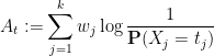
The second half of the proof of Proposition 7 only uses the marginal distributions  and the equation(16), not the actual distribution of , so it can also be used to prove an upper bound on when the exact maximizing distribution is not known, given suitable probability distributions in each variable. The logarithm of the probability distribution here plays the role that the weight functions do in BCCGNSU.
Remark 8 Suppose one is in the situation of (i) and (ii) above; assume the nondegeneracy condition that is positive (or equivalently that is positive). We can assign a “degree”  to each element by the formula

then every tuple in has total degree at most , and those tuples in have degree exactly . In particular, every tuple in has degree at most  , and hence by (17), each such tuple has a -component of degree less than or equal to
  for some with
  . On the other hand, we can compute from (19) and the fact that
  for
for  that
that  . Thus, by asymptotic equipartition, and assuming , the number of “monomials” in of total degree at most is at most
  ; one can in fact use (19) and (18) to show that this is in fact an equality. This gives a direct way to cover by sets
  with
with  , which is in the spirit of the Croot-Lev-Pach-Ellenberg-Gijswijt arguments from the previous post.
We can now show that the rank computation for the capset problem is sharp:
Proposition 9 Let  denote the space of functions from
  to
to  . Then the function
  from
from  to , viewed as an element of
 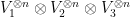 , has rank
  as , where
  is given by the formula

with

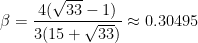
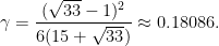
Proof: In  , we have


Thus, if we let  be the space of functions from to (with domain variable denoted
  respectively), and define the basis functions


of  indexed by
  (with the usual ordering), respectively, and set
  to be the set

then  is a linear combination of the
  with
with  , and all coefficients non-zero. Then we have
  . We will show that the quantity of (10) agrees with the quantity
  of (20), and that the optimizing distribution is supported on , so that by Proposition 6 the rank of
  is
is  .
.
To compute the quantity at (10), we use the criterion in Proposition 7. We take  to be the random variable taking values in that attains each of the values
  with a probability of
  , and each of
  with a probability of
  ; then each of the
  attains the values of
  with probabilities
  respectively, so in particular
  is equal to the quantity in (20). If we now set
  and
and

we can verify the condition (16) with equality for all  , which from (17) gives
  as desired.
This statement already follows from the result of Kleinberg-Sawin-Speyer, which gives a “tri-colored sum-free set” in  of size
  , as the slice rank of this tensor is an upper bound for the size of a tri-colored sum-free set. If one were to go over the proofs more carefully to evaluate the subexponential factors, this argument would give a stronger lower bound than KSS, as it does not deal with the substantial loss that comes from Behrend’s construction. However, because it actually constructs a set, the KSS result rules out more possible approaches to give an exponential improvement of the upper bound for capsets. The lower bound on slice rank shows that the bound cannot be improved using only the slice rank of this particular tensor, whereas KSS shows that the bound cannot be improved using any method that does not take advantage of the “single-colored” nature of the problem.
We can also show that the slice rank upper bound in a result of Naslund-Sawin is similarly sharp:
Proposition 10 Let denote the space of functions from  to
to  . Then the function
  from
from  , viewed as an element of , has slice rank
Proof: Let  and
and  be a basis for the space of functions on
  , itself indexed by
  . Choose similar bases for
  and
and  , with
  and
and  .
.
Set  . Then
  is a linear combination of the with , and all coefficients non-zero. Order
  the usual way so that is an antichain. We will show that the quantity of (10) is
  , so that applying the last statement of Proposition 6, we conclude that the rank of is
  ,
,
Let be the random variable taking values in that attains each of the values  with a probability of
  . Then each of the
  attains the value with probability and with probability
  , so
, so

Setting  and
and  , we can verify the condition (16) with equality for all , which from (17) gives
  as desired.
We used a slightly different method in each of the last two results. In the first one, we use the most natural bases for all three vector spaces, and distinguish from its set of maximal elements . In the second one we modify one basis element slightly, with  instead of the more obvious choice
  , which allows us to work with instead of
  . Because is an antichain, we do not need to distinguish and . Both methods in fact work with either problem, and they are both about equally difficult, but we include both as either might turn out to be substantially more convenient in future work.
Proposition 11 Let  be a natural number and let
  be a finite abelian group. Let be any field. Let
  denote the space of functions from to .
Let  be any -valued function on
  that is nonzero only when the elements of
  form a -term arithmetic progression, and is nonzero on every -term constant progression.
Then the slice rank of is  .
.
Proof: We apply Proposition 4, using the standard bases of . Let be the support of . Suppose that we have orderings on such that the constant progressions are maximal elements of and thus all constant progressions lie in . Then for any partition  of , can contain at most
  constant progressions, and as all constant progressions must lie in one of the , we must have
  . By Proposition 4, this implies that the slice rank of is at least . Since is a
  tensor, the slice rank is at most , hence exactly .
So it is sufficient to find orderings on such that the constant progressions are maximal element of . We make several simplifying reductions: We may as well assume that consists of all the -term arithmetic progressions, because if the constant progressions are maximal among the set of all progressions then they are maximal among its subset . So we are looking for an ordering in which the constant progressions are maximal among all -term arithmetic progressions. We may as well assume that is cyclic, because if for each cyclic group we have an ordering where constant progressions are maximal, on an arbitrary finite abelian group the lexicographic product of these orderings is an ordering for which the constant progressions are maximal. We may assume  , as if we have an
  -tuple of orderings where constant progressions are maximal, we may add arbitrary orderings and the constant progressions will remain maximal.
So it is sufficient to find orderings on the cyclic group  such that the constant progressions are maximal elements of the set of -term progressions in in the -fold product ordering. To do that, let the first, second, third, and fifth orderings be the usual order on
  and let the fourth, sixth, seventh, and eighth orderings be the reverse of the usual order on .
Then let  be a constant progression and for contradiction assume that
  is a progression greater than in this ordering. We may assume that
 ![{c \in [0, (n-1)/2]}](https://s0.wp.com/latex.php?latex=%7Bc+%5Cin+%5B0%2C+%28n-1%29%2F2%5D%7D&bg=ffffff&fg=000000&s=0&c=20201002) , because otherwise we may reverse the order of the progression, which has the effect of reversing all eight orderings, and then apply the transformation
, because otherwise we may reverse the order of the progression, which has the effect of reversing all eight orderings, and then apply the transformation  , which again reverses the eight orderings, bringing us back to the original problem but with
 ![{c \in [0,(n-1)/2]}](https://s0.wp.com/latex.php?latex=%7Bc+%5Cin+%5B0%2C%28n-1%29%2F2%5D%7D&bg=ffffff&fg=000000&s=0&c=20201002) .
.
Take a representative of the residue class  in the interval
 ![{[-n/2,n/2]}](https://s0.wp.com/latex.php?latex=%7B%5B-n%2F2%2Cn%2F2%5D%7D&bg=ffffff&fg=000000&s=0&c=20201002) . We will abuse notation and call this . Observe that
. We will abuse notation and call this . Observe that 
 , and
, and  are all contained in the interval
 ![{[0,c]}](https://s0.wp.com/latex.php?latex=%7B%5B0%2Cc%5D%7D&bg=ffffff&fg=000000&s=0&c=20201002) modulo . Take a representative of the residue class
modulo . Take a representative of the residue class  in the interval . Then
  is in the interval
 ![{[mn,mn+c]}](https://s0.wp.com/latex.php?latex=%7B%5Bmn%2Cmn%2Bc%5D%7D&bg=ffffff&fg=000000&s=0&c=20201002) for some
for some  . The distance between any distinct pair of intervals of this type is greater than
  , but the distance between and is at most , so is in the interval . By the same reasoning,
  is in the interval . Therefore
  . But then the distance between and
  is at most , so by the same reasoning is in the interval . Because is between and , it also lies in the interval . Because is in the interval , and by assumption it is congruent mod to a number in the set greater than or equal to , it must be exactly . Then, remembering that and lie in , we have
  and
and  , so
, so  , hence
  , thus
  , which contradicts the assumption that
  .
.
In fact, given a -term progressions mod and a constant, we can form a -term binary sequence with a for each step of the progression that is greater than the constant and a for each step that is less. Because a rotation map, viewed as a dynamical system, has zero topological entropy, the number of -term binary sequences that appear grows subexponentially in . Hence there must be, for large enough , at least one sequence that does not appear. In this proof we exploit a sequence that does not appear for .

.
at most
,
and
.
at most
as a subspace of
for
, such that
, where
is the obvious pairing.


and a finite quantity
, such that
whenever
, and such that
. (In particular,
with
.)


19 comments
Comments feed for this article
24 August, 2016 at 9:38 am
Lior Silberman
In Lemma 1(iii), the first $\latex \oplus$ should be a
[Corrected, thanks – T.]
24 August, 2016 at 12:47 pm
Anonymous
Is it possible to formulate (at least part of) these result in terms of some appropriate notions of entropy and information ?
26 August, 2016 at 11:04 am
Anonymous
i.e. is there an “information theoretic” approach to the notion of “slice rank” and to these results?
26 August, 2016 at 11:10 am
Terence Tao
I don’t think there is a direct information-theoretic interpretation of slice rank for any fixed dimension, but when considering the slice rank of a tensor power in the limit
  it seems that the asymptotic (normalised) slice rank has an information-theoretic interpretation. Right now we can only formalise this in the case that
  has a representation in terms of suitable basis vectors in which the nonzero coefficients are restricted to an antichain (see Proposition 6), but this connection may well hold in greater generality (maybe involving some “noncommutative” version of entropy?).
26 August, 2016 at 5:52 pm
Will
You can interpret the combinatorial problem appearing in Proposition 4 as a particular kind of information problem, where Alice knows a k-tuple of solutions to a problem and must send a message to Bob in the minimum amount of space, and then Bob must give one of the k possible solutions (and Alice and Bob both know the set of possible problems and agree on a communication protocol beforehand). Here S_1,…,S_k are sets of possible solutions and Gamma is the set of possible problems. I don’t know much about this kind of information problem, other than the asymptotic formula in Proposition 6.
Surely something more can be said about this combinatorial problem. But, as Terry says, it’s hard to connect it to slice rank, outside this very special antichain case.
24 August, 2016 at 3:40 pm
Jhon Manugal
tensor products of vector spaces can describe entangled quantum states, as in these notes of Barton Zweibach http://ocw.mit.edu/courses/physics/8-05-quantum-physics-ii-fall-2013/lecture-notes/MIT8_05F13_Chap_08.pdf
24 August, 2016 at 3:45 pm
Hai Le
In the Proposition 9, there seems to be a typo at 1-(x+y+z)^2 = (1-x^2)-y^2-z^2+xy+yz+zx.
24 August, 2016 at 3:47 pm
Hai Le
I was wrong, forgot that it is in F_3
25 August, 2016 at 3:14 am
Matjaž Gomilšek
There is a missing just before “will be called rank one functions,”
[Corrected, thanks – T.]
26 August, 2016 at 6:23 am
Parminder Singh
Do you ever get bored doing mathematics? If no, Why not? If yes, What pushes you again to do it?
30 August, 2016 at 1:36 pm
Yuval Filmus
In (7), the direction of the inequality seems wrong. Also, the word “holds” is missing right after (7).
[Corrected, thanks – T.]
7 September, 2016 at 8:42 am
Paul Gustafson
I think there’s a typo in your comparison with the usual notion of tensor rank, “giving a rank that is greater than or equal to the slice rank studied here”
That should be a “less than or equal,” since there are more rank 1 functions for the usual tensor rank than for the slice rank.
7 September, 2016 at 9:40 am
Will
It is correct. There are actually fewer rank-one functions for the usual tensor rank than for the slice rank, not more as you say. Rank-one functions for the usual tensor rank must split into independent functions of each factor, whereas for slice rank they must only split into a function of one factor times a function of all the other factors.
7 September, 2016 at 6:21 pm
Paul Gustafson
Oh, that makes sense. My mistake!
9 September, 2016 at 9:48 am
Introduction to the polynomial method (and other similar things) | Short, Fat Matrices
[…] polynomial method has made some waves recently (see this and that, for instance), and last week, Boris Alexeev gave a very nice talk on various applications of this […]
16 March, 2017 at 1:00 am
Dion Gijswijt
The set in the proof of Proposition 7 is not convex in general. I think what you need is that
  is convex.
Nice proof!
[Corrected, thanks – WS.]
15 May, 2017 at 1:40 am
Notes of the seminar ‘On the slice rank of functions’ | Points And Lines
[…] of geometrical way. Most, if not all, of the theory can be developed for general tensors (see again Terry’s blog), but we will restrict ourselves to to a special case, which we will explain in the next paragraph. […]
5 March, 2021 at 7:23 am
gowers
A bit late to the party here, but in the statement and proof of Proposition 9, is a typo for
  ?
?
[Corrected, thanks – T.]
15 March, 2023 at 1:34 pm
Sets of points meeting each subspace in a few points | Anurag's Math Blog
[…] of just an affine subspace and many new results have been obtained using the various notions of ranks of a tensor (see this and the references […]